Simple & Multiple Linear Regression
The first conditional model — OLS as orthogonal projection, Gauss–Markov's BLUE property, the Wilks-specialized F-test, and the diagnostic anchors that motivate Topic 22's GLM machinery.
21.1 From Predictions to Lines
Every scatter plot invites a line. A biologist plots height against age and wants to know how growth rate depends on sex. An economist plots a firm’s revenue against advertising spend and wants the marginal return. A machine-learning engineer plots validation loss against training-set size and wants to extrapolate. In all three cases the question is the same: given paired observations , what linear function of best explains — and how much of the variation in is it actually explaining?
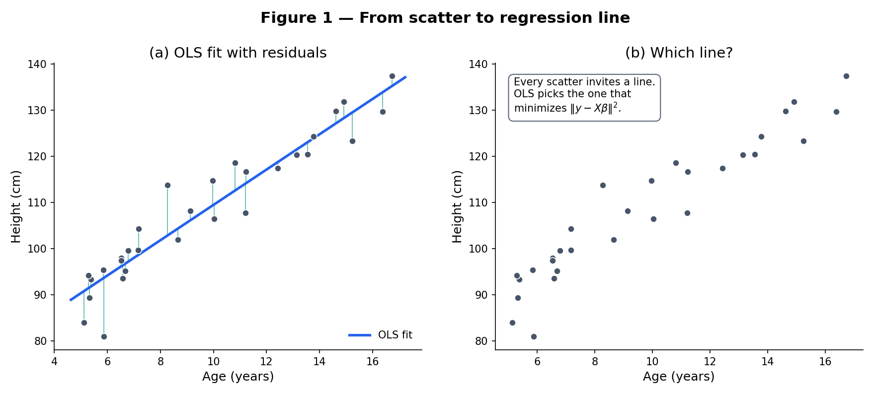
The classical answer — ordinary least squares (OLS) — picks the line that minimizes the sum of squared vertical distances from each point to the line. That choice is not arbitrary. It has a geometric meaning (the residual vector lies orthogonal to the column space of the design matrix), a probabilistic meaning (it is the maximum-likelihood estimator under Normal errors), and an optimality property (Gauss–Markov: among all linear unbiased estimators, OLS has the smallest variance). Topic 21 builds all three in turn.
Given paired data with the treated as fixed (non-random), the simple linear regression model asserts
where are unknown parameters (the intercept and slope) and the errors are random variables with and for all . The errors are assumed uncorrelated: for .
Galton’s 1886 study of hereditary stature plotted adult-child height against mid-parent height and found the regression line’s slope was less than 1 — tall parents tended to have tall children, but on average less tall than the parents. He called this “regression toward mediocrity” (later softened to “regression toward the mean”). Figure 1 shows the Galton-style scatter; the fit line has slope , cutting through the 45° line at the sample mean. The vertical segments are residuals — the part of each child’s height unexplained by the parental-height linear model.
The model is a linear regression: the response depends linearly on the unknown parameters , even though and are nonlinear transformations of the predictor. The matrix form of §21.4 accommodates any such design matrix. What this topic does not cover is nonlinear regression — models like where enters nonlinearly. Those require iterative fitting (Gauss–Newton, Levenberg–Marquardt) and belong to Topic 22 or later.
The word “regression” comes from Galton’s 1886 observation. A century earlier, Legendre (1805) and Gauss (1809, GAU1823) had introduced least squares for astronomical-orbit estimation. The two traditions — Galton’s statistical “regression toward the mean” and Gauss’s computational least-squares — merged into the modern discipline in the early 20th century, with Fisher’s 1922 foundational paper on estimation theory providing the bridge.
21.2 The Least-Squares Criterion
What does “best fit” mean? OLS picks the line that minimizes the sum of squared residuals. For simple regression:
Given data , the sum-of-squared-residuals loss is
The OLS estimator is the minimizer of over .
Squared loss is not the only option — absolute deviation (LAD / quantile regression) and Huber loss are standard alternatives — but OLS has three properties its competitors lack, and one of them is the featured theorem of this topic.
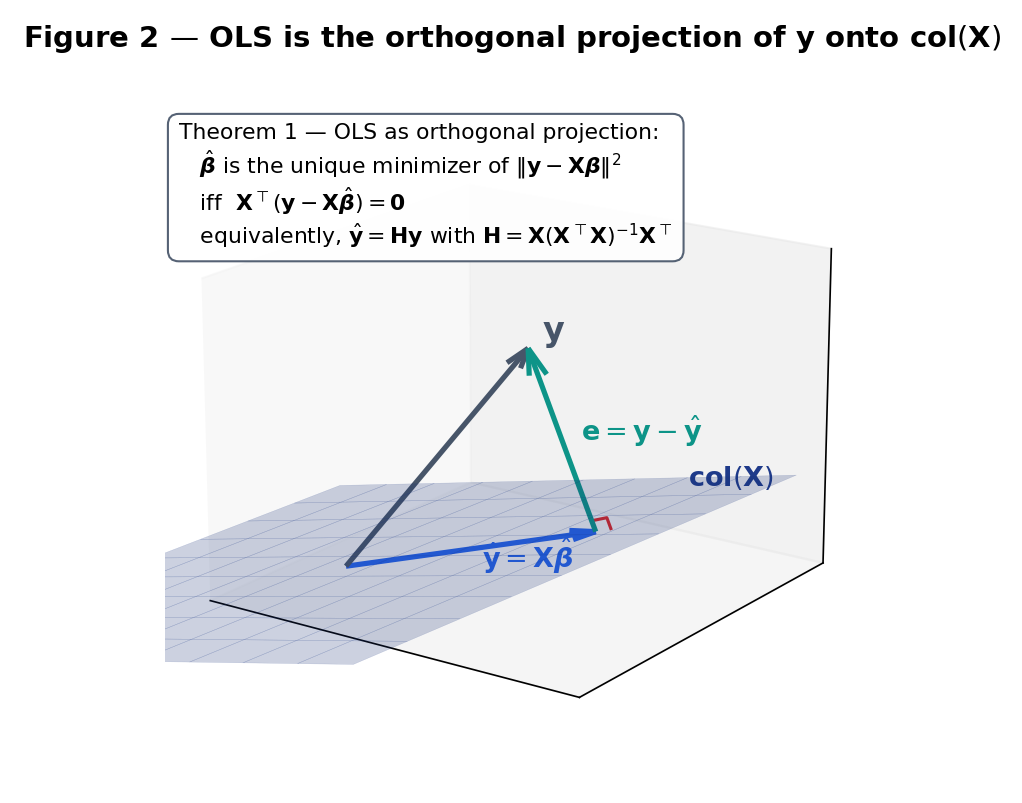
In the simple-regression setup, let denote the fitted values (vectors in ). The OLS solution is the unique pair for which the residual vector satisfies
Equivalently, is orthogonal to the column space , and is the orthogonal projection of onto that subspace. The OLS solution is unique whenever is not constant.
Proof Proof 1 — OLS as orthogonal projection [show]
Setup. Let with the design matrix. is a positive-semidefinite quadratic form in , so a minimizer exists by continuity and coercivity.
First-order condition. Expanding and differentiating,
Setting the gradient to zero at yields the normal equations
Geometric reading. The normal equations say the residual is orthogonal to every column of , hence to every vector in the column space . Since lies in , we have decomposed with and — the defining property of the orthogonal projection onto . Figure 2 renders the picture.
Uniqueness via Pythagoras. For any alternative , write . Then
The two summands on the right are orthogonal: is the residual and , so the cross term vanishes. By Pythagoras,
Hence , with equality iff . When has full column rank (the simple-regression case when is non-constant), this forces . ∎ — using positive-definite quadratic minimization and uniqueness of orthogonal projection onto a closed subspace
Solving the normal equations in the simple-regression case gives the closed form
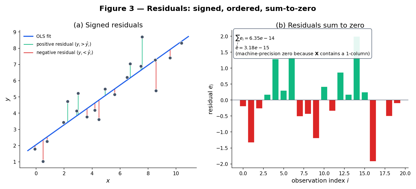
Take the data , . Then , , , , so
The fitted line produces residuals , which sum to (≈ 0, the small numerical residual from finite arithmetic) and have the signature of an OLS fit: one-half positive, one-half negative, approximately centered on zero.
Drag any point or press Tab then arrow keys to nudge. The line is the least-squares fit; the grey segments are residuals; the bar panel shows signed residuals in observation order.
Three reasons, in order of historical importance. (1) Analytic tractability: squared loss is differentiable and convex, so the minimizer has a closed form via the normal equations. Absolute-deviation loss is neither — LAD requires iterative linear programming or specialized algorithms. (2) Normal-errors connection: under Gaussian , OLS coincides with the MLE (see §21.5 Rem 9). (3) Optimality certificate: Gauss–Markov (§21.6) shows OLS is BLUE under second-order assumptions — no competitor in the linear-unbiased class beats it on variance. The forward-pointer cost is sensitivity to outliers: squared loss magnifies large residuals quadratically, so one bad observation can swing the fit. Topic 15’s M-estimators (Huber, Tukey) trade some of Gauss–Markov’s optimality for robustness; the forward pointer in §21.9 Rem 20 states this explicitly.
If we add the stronger assumption , the log-likelihood is
Maximizing over for any fixed is identical to minimizing the sum of squared residuals — OLS and MLE pick the same . Full treatment in §21.5 Rem 9 via Topic 14’s MLE machinery.
21.3 Properties of Simple OLS
With the OLS estimator in hand, we can ask: how well does recover the true ? What fraction of variation in does the fitted line explain? These are the first questions a practitioner asks, and their answers set up the inferential machinery of §21.5 and §21.8.
Given OLS estimates , define
The coefficient of determination is , interpreted as the fraction of total variation in explained by the linear fit.
Under Definition 1 (fixed , zero-mean uncorrelated errors with common variance ),
Brief derivation. Substituting into the closed form,
(The and terms cancel because .) Taking expectations: . The variance: . ∎
Continuing Example 2 with assumed known for illustration at : , so . A 95% Wald CI for is . In practice is unknown and we plug in with a t-distribution critical value — see §21.8. The test–CI duality of Topic 19 tells us this CI is exactly the set of values a two-sided level-0.05 t-test would not reject.
is the fraction of -variance captured by the linear fit. means perfect fit; means the fit is no better than the constant . Two caveats. First, always increases when predictors are added (the enlarged column space cannot shrink the projection’s accuracy), so it is useless as a model-comparison tool across models of different dimension. The adjusted , , penalizes for predictor count but is still ad hoc; principled model selection lives in Topic 24 AIC/BIC/CV. Second, high does not imply the model is correct — the Anscombe quartet of Example 10 exhibits for four datasets with wildly different residual structures, only one of which is actually well-modeled by a line. Residual diagnostics (§21.9) are non-negotiable.
The sample Pearson correlation is related to the slope by and to by (in simple regression). But correlation is symmetric () while regression is directional — the slope of on is not the reciprocal of the slope of on unless . Regression asks “how does depend on ?”, a conditional-expectation question; correlation asks “how much do and co-vary?”, a joint-distribution question.
21.4 The Matrix Form
Simple regression (, single predictor) is the pedagogical on-ramp; the real payoff is multiple regression with predictors plus an intercept. The matrix form unifies every result from §21.2–§21.3 into a single geometric picture that generalizes without change.
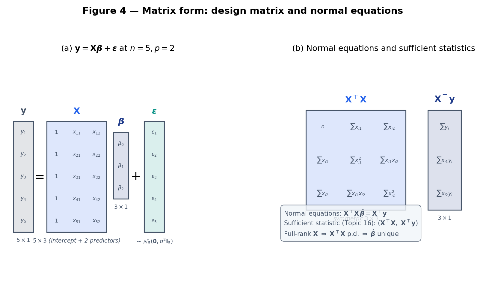
Notation. Throughout this topic and Track 6, we use column vectors by default: are column vectors; their transposes are row vectors. Transposes are written (not ). Vectors are bold lowercase; matrices are bold uppercase. The sample size is ; denotes the number of non-intercept predictors, so the design matrix is with a leading column of ones, and the residual-degrees-of-freedom is . Inner products are ; . For symmetric positive-semidefinite we write ; means is PSD.
Given observations with non-intercept predictors, the design matrix is with a leading column of ones and -th row . The parameter vector collects intercept and slopes. The error vector has and . The linear regression model is
Assuming has full column rank , the OLS estimator minimizing is the unique solution to the normal equations
explicitly given by .
Brief derivation. Differentiating and setting the gradient to zero gives , i.e., . Full column rank makes invertible, so the solution is unique. Proof 1 of §21.2 verified that this critical point is the global minimum via Pythagorean uniqueness. ∎
For simple regression (, so has columns ):
Solving by hand (apply the matrix inverse) reproduces
matching §21.3. The sufficient pair is all the data tells OLS — no other aspect of matters for the point estimate. This discharges the bullet in Topic 16 §16.12: OLS is a function of a Normal-linear-model sufficient statistic.
exists if and only if has full column rank — equivalently, no predictor is a linear combination of the others. When this fails (perfect collinearity), the normal equations have infinitely many solutions and OLS is undefined. In practice even near-collinearity (multicollinearity) destabilizes : variances inflate, standard errors explode, individual coefficients become uninterpretable. The classical diagnostic is the variance inflation factor (VIF); the classical remedy is ridge regression (Topic 23). For Topic 21 we assume full column rank throughout.
When are jointly multivariate Normal with mean and covariance , Topic 8 §8.4 shows the conditional expectation is exactly linear:
So for jointly Normal data, multiple regression is not an approximation — it recovers the population regression line exactly. For non-Normal data, OLS is fitting the best linear approximation to in mean-squared-error, which may or may not be the true conditional mean. The Gauss–Markov theorem (§21.6) handles the “best” part; Rem 11 under Normality promotes it to “unique UMVUE.”
21.5 Distributional Theory under Normal Errors
Gauss–Markov does not require Normal errors — only zero mean, uncorrelated, common variance. But for exact distributional statements — t-tests for individual coefficients, F-tests for nested models, confidence intervals — we need more. The standard additional assumption is Normality.
The Normal linear model extends Definition 4 with the distributional assumption
i.e., the errors are iid . The design matrix remains fixed (non-random).
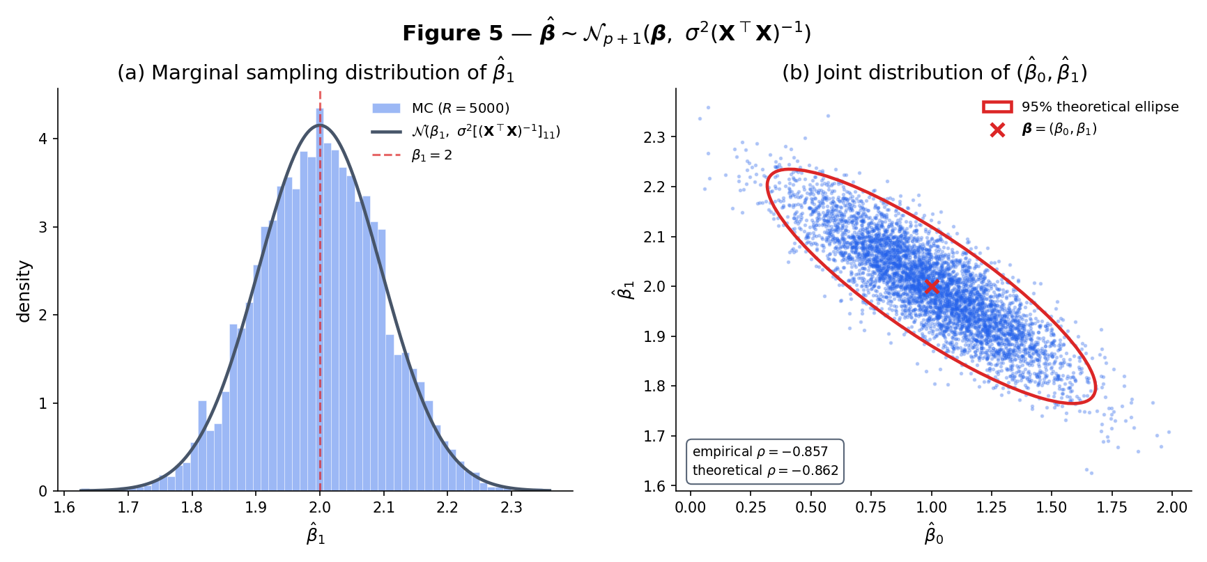
Under Definition 5 (Normal linear model, full column rank),
Brief derivation. is a linear combination of , which is multivariate Normal under the Normal linear model. Linear combinations of MVN vectors are MVN, so is MVN with mean and covariance . ∎
Under the Normal linear model, let . Then
Brief derivation. Write and where is the hat matrix (§21.7). Both are linear functions of ; their cross-covariance is
because (the defining property of the hat matrix). Uncorrelated Normal vectors are independent, so , hence .
For the distribution: . The matrix is symmetric idempotent with rank (see §21.7 Thm 7). A symmetric idempotent quadratic form in iid entries is where is the rank — this is a classical application of the Fisher–Cochran decomposition, cited from Topic 16 Ex 21. Hence . ∎
The Normal log-likelihood is . For any , the that maximizes is the one that minimizes — exactly the OLS problem. So . The MLE of is (biased downward by a factor ); the unbiased of Theorem 5 divides by instead. See Topic 14 for the general MLE framework.
Combining Theorems 4 and 5: for each coefficient ,
The numerator is ; the denominator is , independent of the numerator. Their ratio is Student’s . This pivotal quantity is the foundation of §21.8’s confidence intervals and hypothesis tests — the direct inheritor of Topic 17 §17.7’s one-sample t-test.
21.6 The Gauss–Markov Theorem
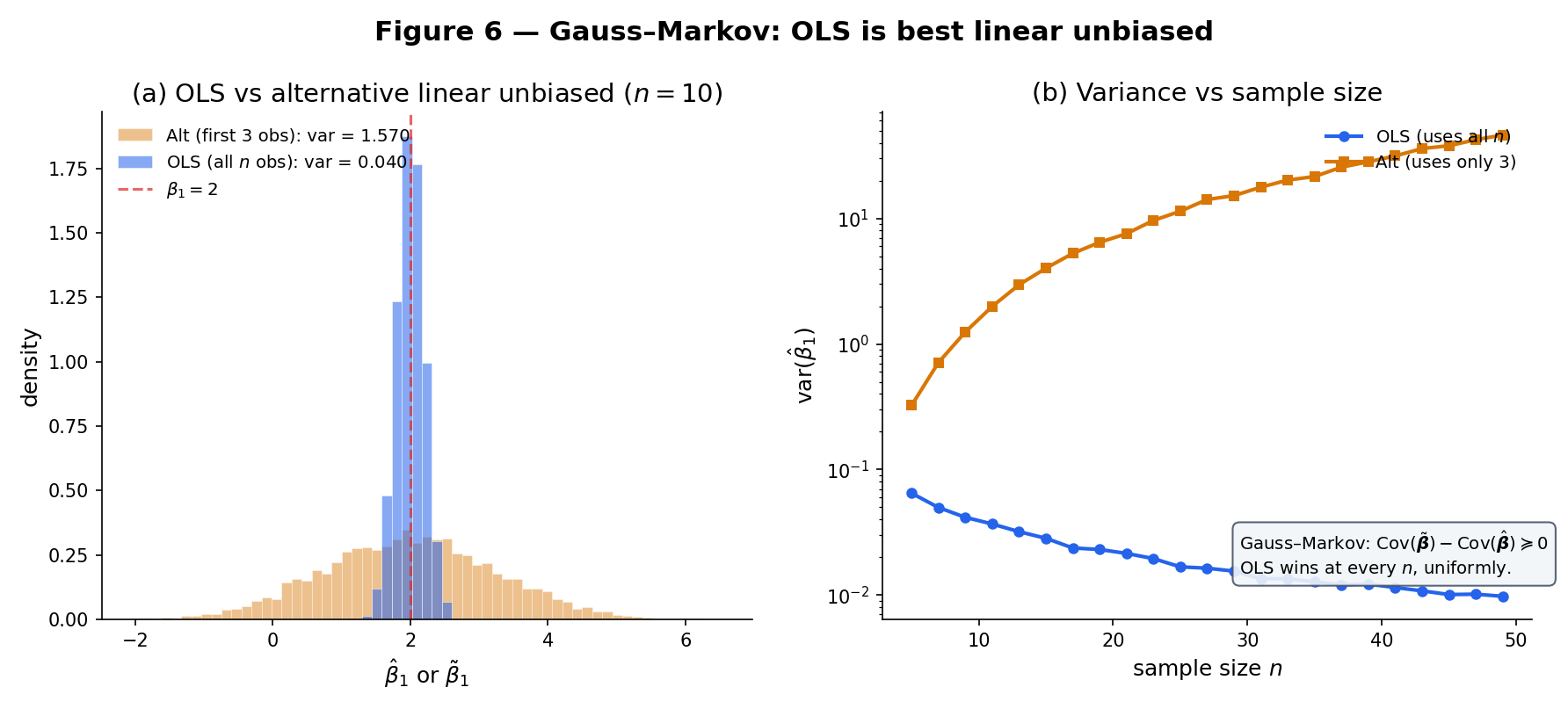
OLS is unbiased and has a tractable sampling distribution. Is it also good? Gauss and Markov together answer: among all linear unbiased estimators of , OLS has the smallest variance. This optimality certificate is the second pillar of the topic, and — unlike the distributional results of §21.5 — it does not require Normality.
An estimator is a linear estimator of . It is unbiased if for all — equivalently, . Among all linear unbiased estimators, the Best Linear Unbiased Estimator (BLUE) is the one with the smallest covariance matrix in the PSD sense: for every competing .
Under Definition 4 (the linear regression model with , , full column rank ) — without any Normality assumption — the OLS estimator is BLUE.
Proof Proof 6 — Gauss–Markov [show]
Setup. Assume , . No Normal assumption.
Linear form. Any linear estimator of has the form for some matrix .
Unbiasedness constraint. . For this to equal for every , we need
Decomposition. Write for some matrix . The unbiasedness constraint becomes
so . This is the load-bearing identity.
Covariance expansion. The covariance of a linear estimator is . Expanding:
The last two cross-terms vanish by (and its transpose ). Therefore
Comparison. Multiplying by ,
Since (any matrix times its transpose is PSD), we have
with equality iff , i.e., .
Scalar corollary. For any linear combination with :
∎ — using unbiasedness to derive ; covariance expansion; PSD property of
Take , , , . OLS gives . A naive competitor — “use only the first three observations to fit a simple regression” — is also linear and unbiased, with . Gauss–Markov guarantees OLS wins; the gap here is a factor of 2.5. Figure 6 shows the full MC comparison.
Gauss–Markov says OLS beats every linear unbiased competitor. Could a nonlinear unbiased estimator do better? Under Normal errors, Topic 16 Thm 4 (Lehmann–Scheffé) answers no: is the unique UMVUE — minimum variance among all unbiased estimators, linear or not — because it is a function of a complete sufficient statistic for the Normal-linear-model exponential family. Without Normality, BLUE is the best we can claim; with Normality, BLUE = UMVUE. This is the §16.12 Track-6 promise discharged.
Gauss–Markov requires only: zero-mean errors, uncorrelated errors, common variance , full column rank . It does not require Normality, independence (only uncorrelatedness), or even identical distribution — errors can follow different distributions as long as they share variance. The one structural assumption that is load-bearing is homoscedasticity: all errors have the same variance. When this fails — heteroscedastic errors, with unequal — OLS is no longer BLUE. The weighted least squares (WLS) estimator reweights observations by and is BLUE in the heteroscedastic setting; see §21.9 Rem 21 for the one-sentence forward pointer to Topic 22.
21.7 Geometry of Fitted Values
Proof 1 of §21.2 identified as the orthogonal projection of onto . That projection has a matrix representation — the hat matrix — and a rich algebraic structure that powers the diagnostic machinery of §21.9.
Under full column rank, the hat matrix is
It “puts the hat on ”: . The diagonal entries are the leverage values of observation — measuring how much the -th observation’s own response contributes to its own fit.
The hat matrix is:
- Symmetric: .
- Idempotent: .
- Rank and trace: .
- Complementary projector: is also symmetric idempotent, with .
Brief derivation. Symmetry: (using symmetry of ). Idempotence: . For rank and trace: a symmetric idempotent matrix has eigenvalues , so its trace equals its rank. Using the cyclic property of trace, . Finally, is symmetric and idempotent (direct check), with trace . ∎
Take , so . Then , , and
Verify: row sums equal 1 (as they must when the first column of is ), trace . The diagonal entries are high — the endpoint observations have the most leverage. The middle observation has , the lowest in this 3-point design.
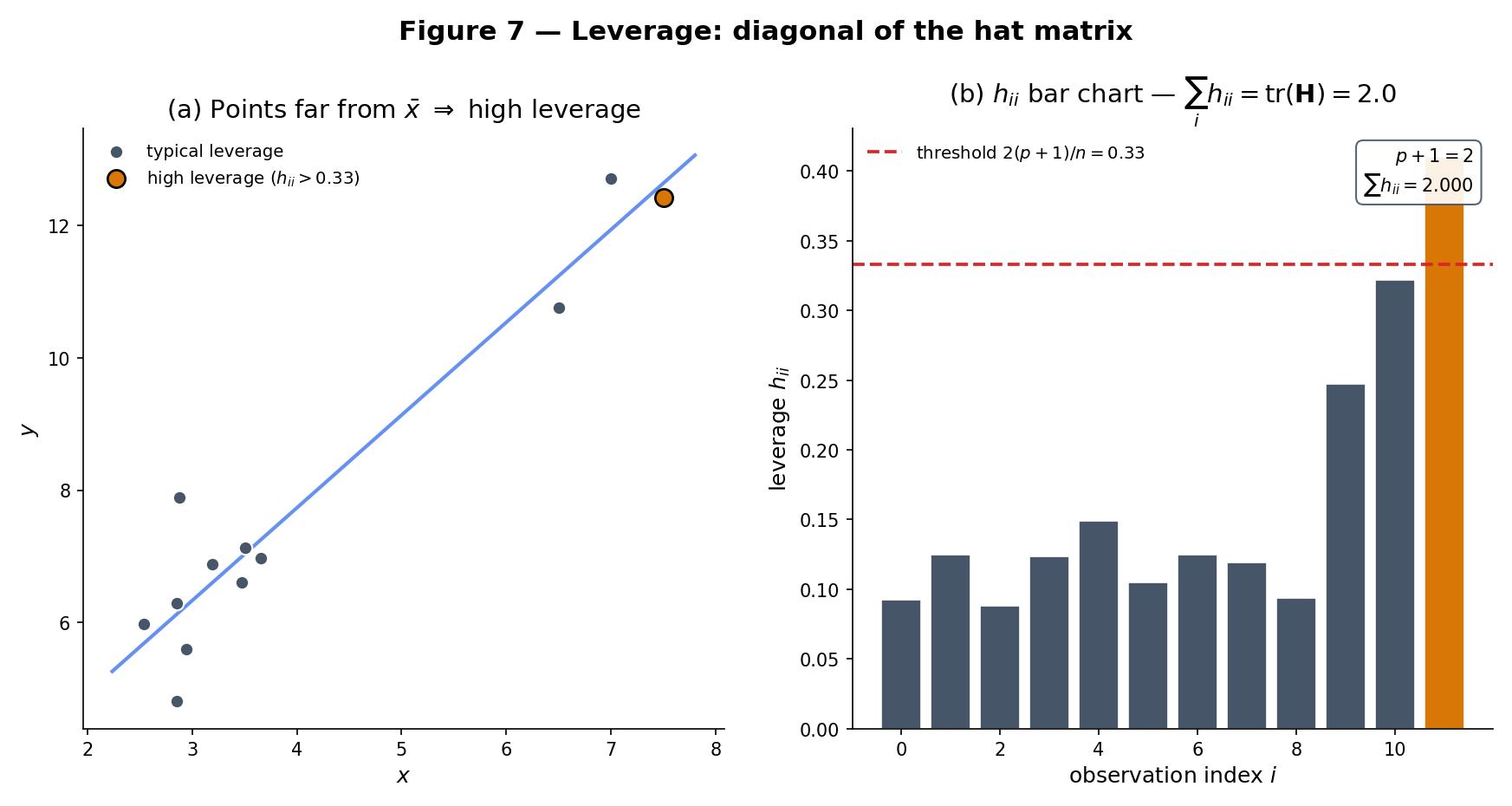
Leverage measures how “far” observation ‘s predictor vector is from the center of the predictor cloud. Since , the average leverage is . The common rule of thumb flags observations with as high-leverage. High leverage is not itself pathological — a well-designed experiment may deliberately include extreme values to reduce — but it is a prerequisite for being influential: an observation with low residual but high leverage contributes little to visible fit quality and much to the estimated coefficients. The diagnostic machinery of §21.9 combines leverage with studentized residuals via Cook’s distance.
The ANOVA identity is the sample analog of Topic 4’s Eve’s law: . The fitted values play the role of the conditional expectation ; the residuals play the role of the conditional deviation. The decomposition is exact in-sample (Pythagoras: when the intercept is included, because ) and is the geometric basis of the one-way ANOVA example in §21.8.
21.8 Hypothesis Tests and Confidence Intervals
The distributional theory of §21.5 plus Topic 19’s test–CI duality delivers the full inferential package: CIs for individual coefficients, tests for nested-model hypotheses, simultaneous inference for families of coefficients.
For the -th coefficient under the Normal linear model, the t-statistic for testing against the two-sided alternative is
Under the Normal linear model and , . Hence a level- two-sided test rejects when , and the corresponding Wald-t confidence interval at level is
Brief derivation. This is Remark 10 restated: the numerator is under . The denominator is with and . Their ratio is standardized over — by definition, . The CI follows from Topic 19 Thm 1: a two-sided t-test and its inversion produce the symmetric interval above. ∎
In a simple regression at , suppose with . Then on . The two-sided p-value is , strongly rejecting the null at conventional levels. The 95% Wald-t CI is — the interval excludes zero, consistent with the rejection.
The individual coefficient test is the simplest case. For nested-model hypotheses — “do these coefficients add anything?” — the t-test generalizes to the F-test, and the F-test has a beautiful interpretation as the finite-sample sharpening of Wilks’ theorem.
Let be the full Normal linear model with parameters and be the reduced model obtained by imposing linear restrictions (so has free parameters). Let be the residual sums of squares under each. Under and Normal errors,
exactly (not just asymptotically).
Proof Proof 9 — F-test as Wilks specialization [show]
Setup. Under , with . The restriction subspace under has dimension ; its orthogonal complement within has dimension .
Independence via Fisher–Cochran. The quadratic forms and project onto orthogonal subspaces of : the residual subspace (dim ) and the restriction-complement subspace (dim ). Topic 16 Ex 21’s Fisher–Cochran theorem says quadratic forms in a Normal vector in orthogonal subspaces are independent.
Chi-squared distributions. (Theorem 5). Under , is a quadratic form in Normal residuals projected onto a -dimensional subspace, hence (Fisher–Cochran on the orthogonal complement).
F-statistic. By definition of the F distribution (Topic 6 Def 13), the ratio of two independent chi-squareds each divided by its degrees of freedom is distributed :
Wilks connection. The log-likelihood-ratio statistic for vs works out to
For large at fixed , by Taylor expansion, so — matching Topic 18 Thm 4 (Wilks). But we just proved that the exact finite-sample distribution of is under Normal errors — not just asymptotically . The F-test is Wilks’ theorem sharpened to an exact distribution under the additional Normal-errors assumption.
∎ — using Topic 18 Thm 4 (Wilks, §18.6), Topic 16 Ex 21 (Fisher–Cochran), Topic 6 Def 13 (F distribution)
Fit a four-predictor model at . To test (predictors 2 and 3 together add nothing), fit both the full and the reduced (two-predictor) models. With , , suppose , . Then on . Since , we reject at ; the p-value is . Predictors 2 and 3 jointly contribute even though, as individual t-tests might show, neither alone is significant at 5%.
Three groups with observations each (). The full model is “group-specific means” — for — fit by an all-dummy design matrix. The reduced model is “common mean” — — fit by a column of ones. The nested F-test has (two group-mean differences), . Its statistic is exactly the classical ANOVA F, and its exact finite-sample distribution under is . Topic 4’s Eve’s law framing is the decomposition:
ANOVA is regression. Topic 21 treats it as a running example rather than a separate chapter.
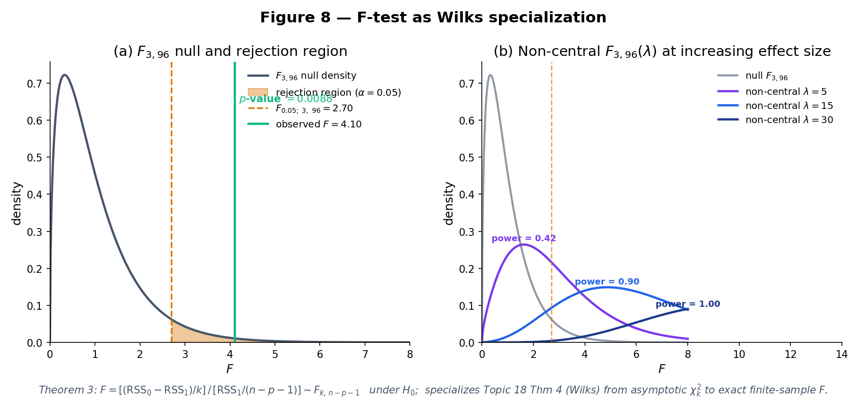
Blue: null F2,46. Amber: non-central F(λ). Grey shading: rejection region of the α-level test.
Topic 19 Thm 1 gave two paths to a CI for any parameter: invert a Wald test (symmetric CI built on ) or invert a LRT (possibly asymmetric CI built by profiling the likelihood). For a coefficient in the Normal linear model, the profile log-likelihood is exactly quadratic — because the log-likelihood itself is quadratic in — so the Wald and LRT inversions produce identical intervals. Under non-Normal errors (GLMs of Topic 22), the profile likelihood is no longer quadratic and the two CIs diverge, with the LRT/profile interval usually better-calibrated. For Topic 21’s Normal linear model: they agree.
A regression report with coefficient CIs at individual level carries a family-wise error rate that grows with . Topic 20 §20.9 Thm 8 hands us the Bonferroni-adjusted CI: widen each interval to individual level and the simultaneous coverage is . This is the default simultaneous-inference tool for regression reports.
For continuous coefficient trajectories — e.g., the fitted regression function evaluated over a grid of — Bonferroni is too conservative (an infinite grid would require infinite widening). The Working–Hotelling (WOR1929) confidence band uses the F-distribution:
The factor replaces Bonferroni’s and delivers exact simultaneous coverage over the entire continuum of values. This discharges the §19.10 closer and the §20.9 Rem 23 forward-pointer.
See §21.8 Rem 15 (Wald vs LRT coincide under Normal errors) and Rem 16 (Bonferroni ⊆ §21.8 simultaneous inference; Working–Hotelling gives continuum bands).
21.9 Diagnostics and Model Validation
All of §21.5–§21.8 assumes the Normal linear model holds. What if it doesn’t? Regression diagnostics are the tools for detecting model failures — heteroscedasticity, non-linearity, outliers, influential points — without which the inferential machinery of the last four sections can produce confident nonsense. The Anscombe quartet (Example 10) is the canonical warning.
Plot on the vertical axis against on the horizontal. Under a correctly specified homoscedastic linear model, the scatter should be structureless — roughly symmetric around the horizontal line , with constant vertical spread across the range of . Three common pathologies: (1) a funnel shape (variance grows or shrinks with ) signals heteroscedasticity; (2) a curved trend signals the linear-in-parameters assumption is missing a quadratic or nonlinear term; (3) one or two extreme points signal outliers or influential observations. If the residual-vs-fitted plot looks random, that is most of the diagnostic battle.
A Q-Q plot of the studentized residuals against theoretical quantiles tests the Normal-errors assumption of Definition 5. Points on the line indicate Normality; systematic departures (S-shaped curves, heavy tails, skew) flag distributional misspecification. Under non-Normal errors the point estimate is still unbiased and Gauss–Markov still applies, but the exact t- and F-distributions of §21.8 become approximations; for moderate this is usually acceptable, but near the tails (extreme p-values, wide CIs) it matters.
When with unequal , OLS coefficient estimates remain unbiased but their standard errors from are wrong — usually too small, producing over-confident inferences. Topic 22 handles this two ways: (1) HC-robust (sandwich) standard errors — White 1980, HC0 through HC3 — replace the homoscedastic SE formula with one that is consistent under arbitrary heteroscedasticity; (2) weighted least squares (WLS) — reweight observations by — delivers BLUE when the are known. Topic 21 surfaces the pathology (Figure 9, RegressionDiagnosticsExplorer) but defers the fix.
An outlier has large residual. A high-leverage point has extreme (large ). An influential point has both, and Cook’s distance
(where is the internally studentized residual) is the standard one-number summary. Thresholds of or flag points whose removal would substantially shift . For robust fitting — M-estimators (Huber, Tukey) that explicitly downweight large residuals — see Topic 15 for the moment-conditions generalization and Topic 22 for robust regression practice.
WLS with known diagonal weights solves the transformed OLS problem where and — classical OLS applied to scaled data. The general case with non-diagonal is generalized least squares (GLS), solving . Both are BLUE in their respective settings — the Gauss–Markov theorem generalizes. Topic 22’s GLM section treats GLS and WLS as special cases of iteratively reweighted least squares (IRLS).
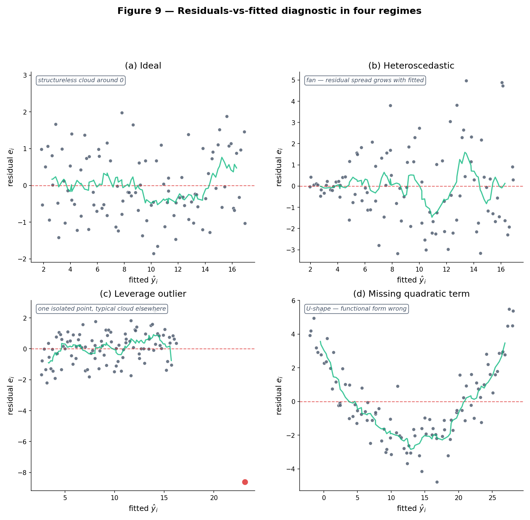
Anscombe (1973) constructed four datasets with identical — every summary statistic rounds to the same value. Yet their residual structures are wildly different: dataset I is a correctly-modeled linear scatter; II is a perfect quadratic with misfit linear model; III has one high-leverage outlier driving a high-leverage fit; IV is a single-x-value cluster plus one vertical outlier. Only dataset I warrants the regression report; the other three require different models or diagnostic intervention. The punchline: no suite of summary statistics is a substitute for looking at the residual plot. The RegressionDiagnosticsExplorer below cycles through five preset scenarios — ideal, heteroscedastic, outlier, non-linear, high-leverage — each producing a distinct residual-vs-fitted, Q-Q, scale-location, and leverage-Cook’s-distance signature. Each failure mode is named, diagnosed, and linked to the appropriate Topic-22/23 remedy.
21.10 Forward Map
Topic 21 built the machinery of the fixed-design homoscedastic Normal linear model. Five directions lead out, and the rest of Track 6 plus Tracks 7–8 plus formalml.com cover them.
The Normal-errors assumption is the restrictive one. Binary outcomes (logistic regression), count outcomes (Poisson regression), positive-skewed outcomes (gamma regression) all fit into the exponential-family GLM framework: a linear predictor composed with a link function such that . The normal equations generalize to iteratively reweighted least squares (IRLS); the F-test generalizes to the deviance test (an exact LRT); HC-robust SEs and GLS both live here.
When is large or is ill-conditioned, OLS variance explodes. Ridge regression adds to the OLS objective, shrinking coefficients toward zero in exchange for bias — a direct bias-variance trade-off controlled by . Lasso uses and produces exactly-zero coefficients (variable selection). Elastic net combines both. Topic 23 covers the penalized objective, coordinate descent solvers, the LARS path, and the cross-validated selection.
Adjusted is a limited criterion. AIC (Akaike) penalizes by ; BIC (Schwarz) by ; cross-validation estimates out-of-sample predictive performance directly, and Stone’s 1977 theorem identifies LOO-CV with AIC asymptotically. Mallows’ is the Gaussian-linear special case. The three criteria diverge in the large- regime: BIC is selection-consistent when the true model is in the candidate set, AIC and CV are minimax-rate optimal for prediction, and Yang 2005 proves the two properties are formally incompatible. Topic 24 develops the full theory.
A conjugate Normal-inverse-gamma prior on yields a closed-form Normal-inverse-gamma posterior, with the posterior mean an explicit ridge-regression estimate (the prior precision plays the role of ). The Bayesian CI is the credible interval — a subset of parameter space with posterior mass — which agrees with the Wald-t CI only under flat priors and as . The conditional-MVN calculation of Topic 8 §8.4 is the mechanical engine. Topic 25 §25.5 covers the scalar Normal–Normal-Inverse-Gamma case; non-conjugate priors are handled via MCMC (Topic 26), with the regression extension developed in Topics 27–28.
When the linearity assumption itself is too restrictive, nonparametric regression estimates without assuming a parametric form. Kernel regression (Nadaraya–Watson), local polynomial regression, and smoothing splines all replace the parametric with a data-driven smooth function. The bias-variance trade-off is controlled by a bandwidth or smoothing parameter; Track 8’s Topic 30 (Kernel Density Estimation) treats the density-estimation theory, and the covariate-conditional (regression) extension is developed at formalml.
Mixed-effects (hierarchical) models add random coefficients for grouped data, handling repeated measurements or nested designs that violate the independent-errors assumption of §21.5. The formalML: Mixed effects topic covers the REML estimator and shrinkage. Causal inference via IV, DiD, RDD, and synthetic control all live in the linear-model framework with identifying restrictions; see formalML: Causal inference methods .
When , OLS fails and penalized methods (Topic 23) become essential. The theory of high-dimensional regression — sparsity rates, minimax bounds, double descent — lives at formalML: High-dimensional regression . The modern regime where with kernel-like implicit regularization (neural networks, random features) is an active research area that Track 8 and formalml.com’s theory topics touch.
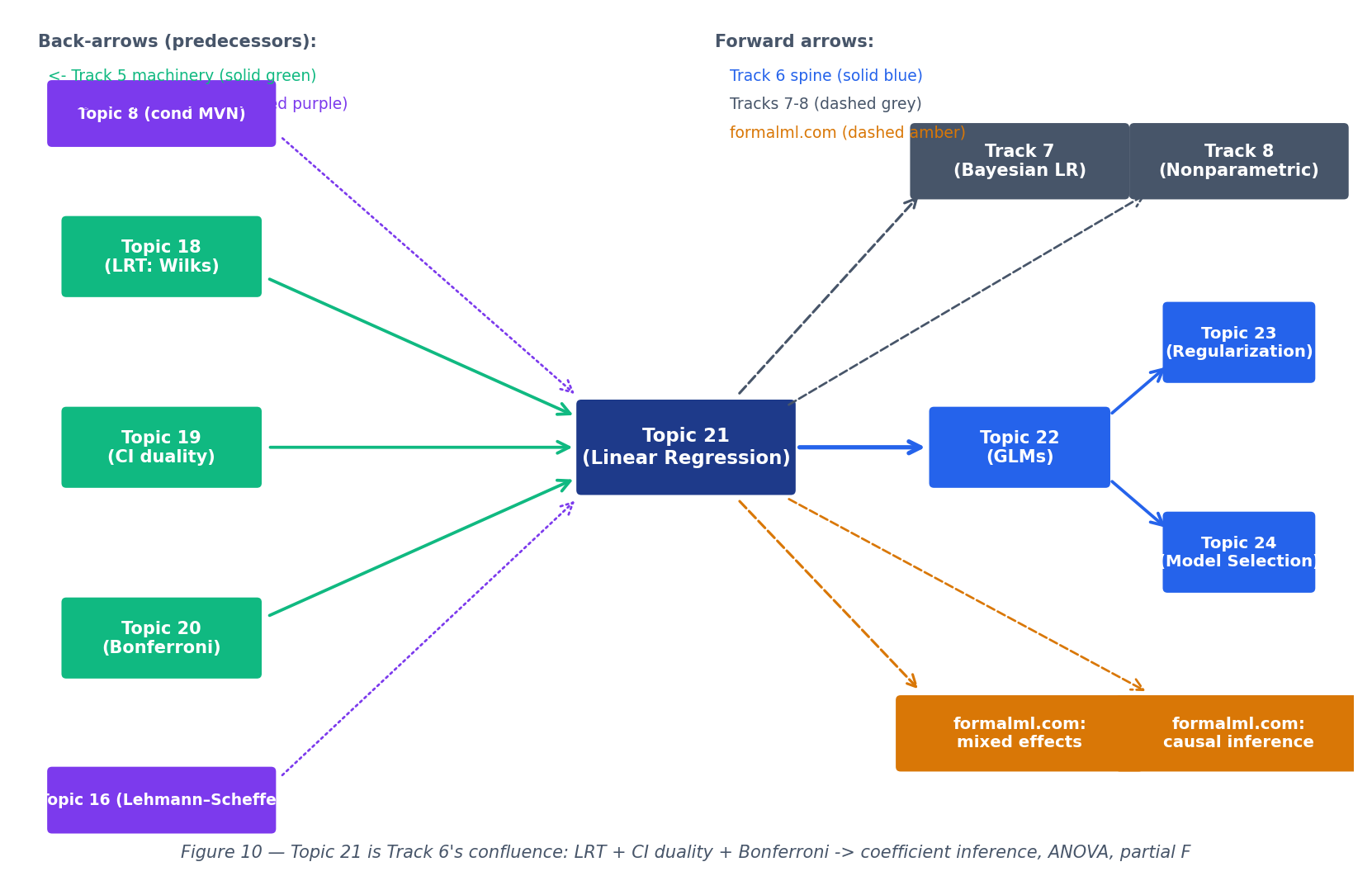
Track 5 closed with simultaneous inference; Track 6 opens with the first conditional model. Every §21.8 result — the F-test, the coefficient CIs, the Bonferroni adjustment, the Working–Hotelling band — is a direct application of Track 5’s machinery to the geometry of §21.2 and §21.7. The next three Track 6 topics widen the scope: GLMs drop the Normal-errors assumption, regularization handles , model selection chooses among nested models. But the orthogonal-projection picture of Proof 1 — residual column space, fitted value as the closest point in the column space — is the geometric anchor that every extension rests on. When in doubt, draw Figure 2 again.
References
- Erich L. Lehmann and Joseph P. Romano. (2005). Testing Statistical Hypotheses (3rd ed.). Springer.
- George Casella and Roger L. Berger. (2002). Statistical Inference (2nd ed.). Duxbury.
- George A. F. Seber and Alan J. Lee. (2003). Linear Regression Analysis (2nd ed.). Wiley.
- Sanford Weisberg. (2005). Applied Linear Regression (3rd ed.). Wiley.
- William H. Greene. (2012). Econometric Analysis (7th ed.). Pearson.
- Holbrook Working and Harold Hotelling. (1929). Applications of the Theory of Error to the Interpretation of Trends. Journal of the American Statistical Association, 24(165A), 73–85.
- Francis Galton. (1886). Regression Towards Mediocrity in Hereditary Stature. Journal of the Anthropological Institute of Great Britain and Ireland, 15, 246–263.
- Carl Friedrich Gauss. (1823). Theoria Combinationis Observationum Erroribus Minimis Obnoxiae. Werke, IV, 1–108.
- Andrey A. Markov. (1900). Wahrscheinlichkeitsrechnung. Teubner.