Maximum Likelihood Estimation
Likelihood function, score equation, consistency, asymptotic normality, efficiency — the workhorse of parametric inference.
14.1 The Likelihood Function
Topic 13 built the machinery for evaluating estimators — bias, variance, MSE, consistency, asymptotic normality, Fisher information, the Cramér–Rao bound. It did not tell us where estimators come from. For specific families we pulled the sample mean and sample variance out of the air and verified their properties. What we need now is a principle — a recipe that takes a parametric model and spits out an estimator with good properties whenever the regularity conditions hold. The likelihood principle is that recipe, and the maximum-likelihood estimator is the estimator it produces.
The idea is disarmingly simple. Suppose we have a parametric family and an iid sample . For any candidate value , the joint density evaluated at the data — — measures how “plausible” that is as a generator of the data we actually observed. Among all candidates, the maximum-likelihood estimator picks the one that makes the data most probable. It is the peak of a landscape indexed by , and everything else in this topic is about that landscape: its shape, its curvature, the rate at which it sharpens as data accumulates, and how to climb it when no closed form is available.
Let be a parametric family of densities (continuous case) or PMFs (discrete case), and let be an observed sample. The likelihood function is the joint density or PMF evaluated at the observed sample, viewed as a function of the parameter with the data held fixed:
When the data are understood we write for short.
The likelihood has the same algebraic form as the joint density, but its role is inverted. The joint density is a function of the data with the parameter fixed — what probability do we assign to different samples under this ? The likelihood is a function of the parameter with the data fixed — how plausible is each in light of the data we observed? The two objects are numerically equal after evaluation, but we read one “across samples” and the other “across parameters.” This inversion is the entire conceptual move of likelihood-based inference.
Two warnings. First, is not a probability density over . It is not normalized, and the parameter is not random in the frequentist setup — it is a fixed (unknown) constant. Calling a “probability of ” is a category error that will mislead you in every Bayesian calculation that follows later. Second, we can always rescale: and for any identify the same maximizer. What matters about the likelihood is its shape, not its height.
The log-likelihood is
It is the sum (not the product) of per-observation log-densities, and it has the same maximizer as because is strictly increasing.
We will essentially never work with directly. The log-likelihood is better behaved in every way that matters: products become sums, the derivative is the score function, the second derivative is the (negative) observed Fisher information, and for exponential families the whole object is concave in the natural parameter. All of the asymptotic theory — consistency, asymptotic normality, efficiency — lives on the log-likelihood, not on the likelihood.
The switch from to is not cosmetic. Three things happen simultaneously, and each is load-bearing.
(1) Products become sums. For iid data is a product of terms; is a sum. Sums are what every limit theorem in probability speaks to — the law of large numbers for sample averages, the central limit theorem for standardized sums. The transition is what lets consistency and asymptotic normality inherit directly from the LLN and CLT applied to .
(2) Concavity (often). For exponential families in the natural parameter, is strictly concave: it has a unique maximizer, and any local maximum is the global one. The likelihood is not concave, just log-concave — a strictly weaker property. Working in log-space is what makes uniqueness and Newton-Raphson convergence arguments tractable.
(3) Numerical stability. Products of many small probabilities underflow to zero in floating point. A sample of Normal observations produces an that is effectively zero — but is a perfectly ordinary number on the order of . Anyone who has fit a model to more than a few hundred data points has implicitly used for this reason alone.
Let be iid with known. The per-observation density is . Taking the product over and then the logarithm:
The first term does not depend on , so we can drop it when maximizing; what remains is the negative sum of squared residuals. Maximizing is therefore the same as minimizing . Least squares and maximum likelihood, for Normal-error models, are the same procedure seen from two angles — one statistical, one geometric.
Let be iid . The PMF is for . Writing for the number of successes,
The likelihood is a polynomial in of degree ; the log-likelihood is linear in and . The shape of — a single peak somewhere between and , concave — is already visible in the formula without any calculus.
Let be iid with density for . Then
Again a clean closed-form log-likelihood, linear in apart from the growth term. For any sample with , is strictly concave in (its second derivative is ), so the maximizer is unique.
14.2 The Maximum Likelihood Estimator
With the log-likelihood in hand, the estimator defines itself.
The maximum-likelihood estimator of is any value that maximizes — equivalently, that maximizes :
When the maximizer is unique, we write . When multiple maxima exist — e.g., on the boundary of , or at non-smooth points — we pick any of them; the finite-sample behavior can differ, but the asymptotic theory is unaffected.
Two things to notice. The MLE is defined as a maximizer, not a root of the score equation: boundary solutions and points where the score is undefined are still MLEs when the global maximum lives there. For the well-behaved cases that dominate practice — compact or open parameter space, smooth , unique interior maximum — the MLE is the unique root of the score equation, which is what Theorem 1 below captures. We will mostly work in this setting and flag boundary complications when they arise.
Suppose is an open interval, is differentiable on , and the global maximizer lies in the interior of . Then satisfies the score equation
where is the per-observation score.
This is calculus: at an interior maximum of a differentiable function, the derivative is zero. Definition 10 in Point Estimation defined and ; the novelty in Topic 14 is that we now solve the score equation for instead of studying its expectation at a fixed . The reader should treat Theorem 1 as a practical recipe: to compute an MLE, write down , differentiate with respect to , set the result to zero, and solve.
The next four examples run this recipe for the four simplest families. They are the workhorses of every applied statistics course, and they are worth deriving cleanly because Topic 14 will invoke them repeatedly.
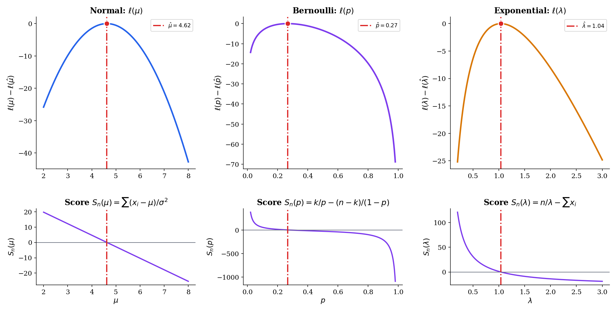
From Example 1, . Differentiating,
Setting the derivative to zero and dividing by gives , so
The second derivative confirms this is a maximum, not a minimum. The MLE of the Normal mean is the sample mean. Every other Topic 13 property of — unbiasedness, variance , asymptotic normality with rate , efficiency — is now a property of the MLE.
From Example 2, with . Differentiating,
Setting this to zero: , so , and therefore , giving
The sample proportion is the MLE — unsurprising in hindsight, and intuitive. The second derivative is for , confirming a maximum. At the boundary or the MLE is or , at the edge of the parameter space — a clean example of a boundary solution.
From Example 3, . Differentiating,
Setting this to zero gives :
Note that the MLE is a nonlinear function of . Because is convex, Jensen’s inequality implies , so the MLE is biased for finite . We will recover bias-free behavior asymptotically, but this is a useful reminder that MLEs are not generally unbiased; they are consistent and asymptotically efficient, not unbiased in finite samples.
For iid data with PMF ,
The final term does not depend on . Differentiating the rest,
and setting this to zero gives . The Poisson MLE is the sample mean — the same estimator as for the Normal mean and the Bernoulli proportion. This is not a coincidence: in each case the natural sufficient statistic is , and the MLE is its normalized version. Exponential families make this pattern universal (Exponential Families, §7.8).
The four examples above all give the MLE as a clean function of the sample mean. That is a feature of their exponential-family structure, not a general property of MLE. For most parametric families — Gamma shape, beta shape, Weibull, Cauchy location, logistic regression, hidden Markov models, neural networks — the score equation has no closed-form solution, and the MLE must be computed numerically. Section 14.7 develops Newton-Raphson for exactly this situation: write down the score and the observed Fisher information, pick a starting value, iterate , and stop when the steps become small. Every optimization method in modern machine learning — SGD, Adam, L-BFGS — is a variation on this theme applied to the log-likelihood or a regularized variant.
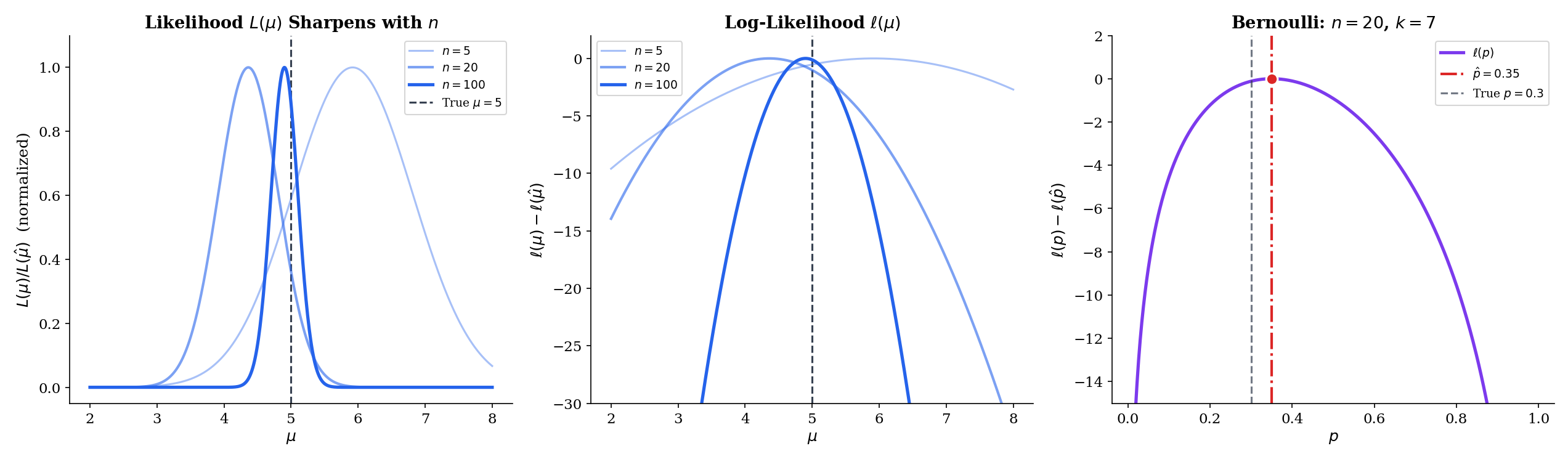
Before moving on, explore the log-likelihood landscape for these four families. The panel below draws a sample of size from the true parameter , plots , and overlays the quadratic approximation together with the 95% Wald confidence interval . Sweep from to and watch the likelihood sharpen — the curvature at the peak (Fisher information) grows linearly with , so the Wald interval shrinks like .
14.3 Functional Invariance
The next property is the one the reader is most likely to have used without ever proving — or even articulating as a theorem.
Let be the MLE of , and let be any function (not necessarily one-to-one). Then the MLE of is
Invariance is what lets you say “the MLE of the standard deviation is the square root of the MLE of the variance” without a separate derivation. It is what lets a neural-network practitioner say “the MLE of the sigmoid-output probability is once we have the MLE of .” It is the glue between the MLE in its natural parameterization and the MLE in whatever parameterization the application requires.
The proof for one-to-one is a change-of-variables argument. Let , so . The likelihood in the new parameterization is , and its maximizer is such that , i.e., . For non-one-to-one , the standard device is the profile likelihood: for each , maximize over , then maximize the result over . Under this definition the invariance property extends without change. Casella & Berger (2002) §7.2.2 gives the detailed argument; the one-to-one case is enough for everything in this topic.
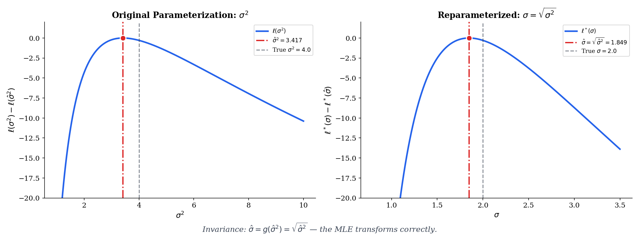
If is the MLE of the Normal variance (as derived from the two-parameter Normal log-likelihood by zeroing the score in ), then by invariance the MLE of the standard deviation is
No separate maximization is needed. Notice that is biased even though would be unbiased if we used instead of ; invariance preserves the MLE but does not preserve unbiasedness under nonlinear transformations. The two properties simply track different things.
In Bernoulli data, the MLE of is . The odds are , a strictly increasing transformation on (so the one-to-one case applies). By invariance, the MLE of the odds is
The odds are the natural parameter of the Bernoulli family: is the logit link that logistic regression uses. Invariance is what makes “logistic regression on ” equivalent to “MLE of then take the log-odds” — the two routes agree at the estimate.
The explorer below shows invariance live: choose a transformation , and watch the MLE on the base scale (left) transport to the MLE on the transformed scale (right). The two panels are two views of the same likelihood, not two separate maximizations.
Invariance transports the point estimate under , but it does not transport the sampling distribution. If , what happens to ? Theorem 7 in Topic 13 (delta method) gives the answer:
So the asymptotic variance scales by . A consequence: the Fisher information transforms tensorially, and efficient estimators in one parameterization remain efficient under smooth reparameterization. Invariance is about the point; the delta method is about the spread.
14.4 Consistency
The first asymptotic property is the most basic. As the sample size grows, does the MLE settle on the true parameter?
Before we can even state consistency, we need a condition that rules out a pathology: two different parameter values giving the same distribution. If for , no amount of data can tell the parameters apart, and no estimator can be consistent.
The family is Kullback–Leibler identifiable at if for every in ,
Equivalently: is the unique maximizer of .
The KL divergence is zero only when the two distributions agree almost surely, so KL-identifiability is the minimal non-degeneracy we need. Every standard parametric family — Normal, Bernoulli, Exponential, Poisson, Gamma, Beta, exponential families in general — is KL-identifiable on its natural parameter space. Non-identifiability shows up in mixture models (label-switching), overparameterized neural networks (many weight configurations realize the same function), and non-identified latent-variable models — all genuine problems that the MLE machinery as stated below does not handle.
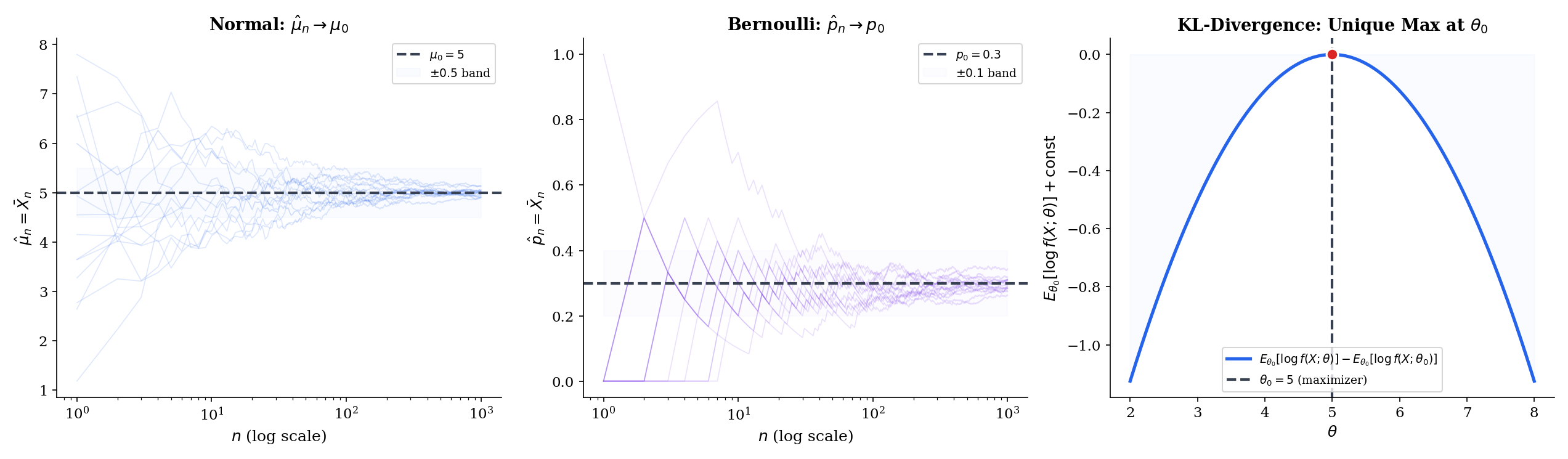
Let be iid from where . Assume (i) is compact, (ii) the family is KL-identifiable at , and (iii) is continuous in for every and dominated by an integrable function. Then the MLE is weakly consistent:
Proof [show]
Define the population log-likelihood
the thing the sample log-likelihood is trying to estimate. By KL-identifiability, is the unique maximizer of : for any ,
This is the Gibbs inequality: the true density maximizes the expected log-likelihood among all densities. By the strong law of large numbers from Topic 10, applied pointwise to the iid sequence at every fixed ,
The next step is the argument that pointwise convergence plus compactness plus continuity upgrades to uniform convergence on :
This is a standard Glivenko–Cantelli-type argument: partition into finitely many small neighborhoods, use pointwise LLN on the centers, and bound oscillations within neighborhoods by the dominating function. Van der Vaart (1998) Theorem 5.7 gives the detailed execution; the only ingredients are the three assumptions above.
Now let and consider the open neighborhood . The complement is compact, so attains its maximum there at some ; by identifiability,
On the event — which has probability tending to one by uniform convergence — any maximizer of must lie in : if it lay outside, then
contradicting the maximality of relative to (for large enough , ). Therefore , i.e., .
The two ingredients are worth abstracting. The Gibbs inequality — , with equality only at — says that the true parameter is the unique maximizer of the population log-likelihood. The LLN says the sample log-likelihood converges to the population log-likelihood. Consistency is just “the argmax of a uniform limit is the argmax of the limit.” Every modern MLE consistency proof is this argument, with different amounts of care invested in the uniform-convergence step for complex parameter spaces.
The three conditions in Theorem 3 — compact , KL-identifiability, continuity with domination — are called regularity conditions. They are standard in most parametric problems, and they can be relaxed in a number of directions:
- Compactness of : Usually replaced by “the MLE eventually lies in a compact subset of with probability one,” which holds under consistency of a coarser preliminary estimator. For open (e.g., for the Normal mean), this is almost always true, but the proof becomes messier.
- Identifiability: Non-negotiable. Label-switching in mixture models, equivalent parameterizations in neural networks, and unobservable components in latent-variable models all violate identifiability in different ways. The MLE in these settings is consistent only for the identified quotient — e.g., the set of mixture distributions, not the parameter vector of component labels.
- Continuity and domination: Continuity of in is almost always immediate. Domination by an integrable function (so expectations are finite and uniform LLN applies) can fail for heavy-tailed families, which is why the MLE story becomes more delicate for Cauchy and similar distributions.
When the conditions hold, they buy you consistency for free — no explicit convergence rate, no finite-sample guarantees, but the estimator does eventually home in on the truth. Rates and finite-sample behavior are the job of asymptotic normality (§14.5) and large-deviations-type bounds (Topic 12).
14.5 Asymptotic Normality
Consistency says converges to . Asymptotic normality says how fast and with what shape. Under regularity, the answer is canonical — the sampling distribution, standardized by , is Gaussian with a variance we can write down exactly.
Let be iid from on an open interval , with the MLE. Assume the conditions of Theorem 3 for consistency, plus (iv) is twice continuously differentiable in a neighborhood of with dominated second derivative, and (v) the Fisher information . Then
Proof [show]
Write for the sample log-likelihood and for the total score. Because maximizes in the interior of (which happens with probability tending to one by consistency) and is twice differentiable, . Taylor-expand around to second order, for some between and :
Solve for :
Multiply both sides by and reorganize:
The numerator is a standardized sum of iid scores. By Theorem 8 in Point Estimation, the score has mean zero and variance under , so the central limit theorem gives
The denominator is the negative of the sample average of second derivatives of the log-density. By consistency ; by the LLN applied to the iid sequence and the dominated continuity of the second derivative,
The last equality is the “information equals negative expected Hessian” identity (Theorem 8 of Topic 13), which in turn relies on the regularity conditions permitting differentiation under the integral sign.
Put the two pieces together with Slutsky’s theorem: a sequence converging in distribution divided by a sequence converging in probability to a positive constant converges in distribution to the ratio of the limits. Thus
The proof shows the MLE as a ratio of two averages — the score and the observed Hessian — each of which has a limit theorem. The CLT handles the numerator; the LLN handles the denominator; Slutsky combines them. This is the template for every M-estimator asymptotic-normality proof: identify the estimating equation, Taylor-expand, apply CLT to the leading term, LLN to the curvature term, and Slutsky to combine. The MLE is the estimating equation , but the same scaffolding works for robust M-estimators, GMM, quasi-likelihood, and many estimators in modern econometrics.
For Normal with known and , (Example 10 of Topic 13). Theorem 4 gives
This is the classical CLT for the sample mean, now recovered as a special case of the general MLE asymptotic-normality theorem. For Normal data, the “asymptotic” normality is actually exact at every finite : for any , not just in the limit. The MLE framework gives one unified result; for this particular family the result happens to hold non-asymptotically.
For Bernoulli with , the Fisher information is , so . Theorem 4 gives
This is the two-sided de Moivre–Laplace theorem in disguise. For a 95% Wald confidence interval we replace by in the asymptotic variance:
This is the formula every introductory statistics class derives ad hoc — it is the MLE Wald interval applied to the Bernoulli family. The interval has known coverage issues near or ; the Wilson score interval and the Agresti–Coull interval are alternatives. What the MLE machinery gives us is the default construction; better intervals require more careful analysis of finite-sample behavior.
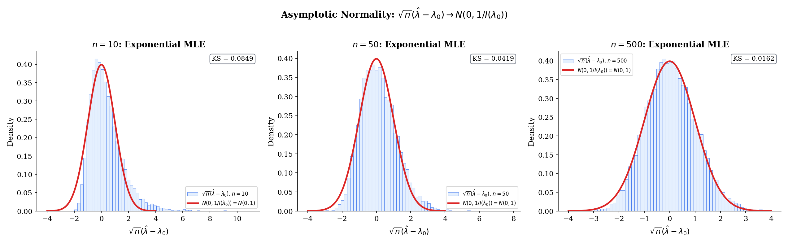
The Monte-Carlo explorer below makes Theorem 4 concrete. For each MC draw, we sample observations from the true parameter, compute the MLE, and add it to a running histogram. Toggle standardized to watch collapse onto — the asymptotic statement in pixels. The readout reports the MC efficiency , which should approach as grows.
The arrow is deceptively clean. In finite samples, three things can go wrong:
(1) Slow convergence near boundaries. For Bernoulli with true near or , the sampling distribution of is very skewed and discrete; the Wald interval undercovers dramatically. The convergence rate is still , but the hidden constants are huge near boundary points.
(2) Bias at second order. The MLE is consistent but generally not unbiased; the bias shrinks at rate , so it is negligible asymptotically but can matter at moderate sample sizes. The classical “Bartlett correction” adjusts likelihood-ratio tests for this second-order bias.
(3) Asymptotic efficiency ≠ finite-sample optimality. At fixed , a biased estimator with smaller variance (e.g., James–Stein in , or a shrinkage estimator) can dominate the MLE in MSE. Asymptotic efficiency says the MLE is optimal as ; for small you may well want to look elsewhere. Topic 13 §13.8 developed this point carefully.
A healthy reading of Theorem 4 is: “for large enough , with well-behaved parameters, you will not be led astray by the Gaussian approximation.” The phrases “large enough” and “well-behaved” are load-bearing and should be checked by simulation whenever is less than a few hundred or the parameter is near a boundary.
Multivariate extension (sidebar)
When is a parameter vector, the same argument runs with the score becoming a gradient and the Hessian becoming a matrix. The Fisher information is the positive semi-definite matrix
and the asymptotic-normality statement becomes
The component-wise Wald CI for the -th parameter is , using the -th diagonal of the inverse Fisher information matrix evaluated at the MLE. The proof is notationally heavier — vector Taylor expansion, matrix Slutsky, continuous-mapping of the matrix inverse — but conceptually identical to the scalar case.
The full multivariate machinery, including the role of the Cramér–Rao matrix inequality and the block structure of information matrices for multi-parameter GLMs, is developed in Topic 21 (Linear Regression) and Topic 22 (Generalized Linear Models).
14.6 Asymptotic Efficiency
Consistency and asymptotic normality locate the MLE within the space of well-behaved estimators. Efficiency ranks it.
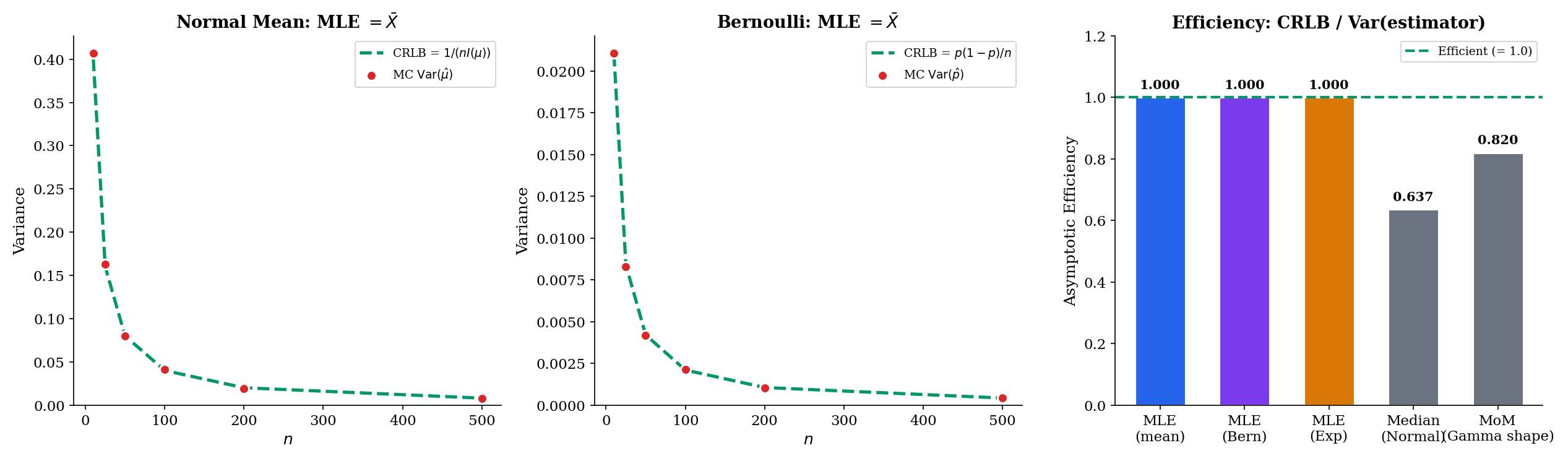
Under the conditions of Theorem 4, the MLE achieves the Cramér–Rao asymptotic variance: its asymptotic variance equals the Cramér–Rao lower bound for the class of regular estimators. In particular, for any other regular asymptotically-normal estimator with ,
Proof [show]
Theorem 9 in Point Estimation — the Cramér–Rao lower bound — proved that any unbiased estimator of satisfies , which in asymptotic-variance language means for its limiting Gaussian spread. The MLE, by Theorem 4 above, has asymptotic variance exactly , which is the CRLB. No regular estimator can do strictly better than the MLE asymptotically.
Efficiency is the statement that no one can beat the MLE asymptotically. In the ML literature, this result is sometimes called the “Cramér–Rao bound saturates at the MLE”: the information inequality turns into an equality for the maximum-likelihood estimator. Every other regular estimator wastes information — extracts less precision from the data than the data actually contains — and the MLE is the unique one (within the regular class, at the first asymptotic order) that does not.
Line up the three workhorse examples:
| Family | MLE | CRLB | Efficient? | ||
|---|---|---|---|---|---|
| Normal, known | Yes (exact at every ) | ||||
| Bernoulli | Yes (asymptotically) | ||||
| Exponential | Yes (asymptotically) |
All three MLEs achieve the CRLB in the limit; the Normal mean achieves it exactly at every finite . Efficiency is not specific to exponential families — it is specific to the MLE — but exponential families make the arithmetic particularly clean because the score is linear in the sufficient statistic.
Theorem 5 says no regular estimator can beat the MLE asymptotically. The catch is the word regular. Joseph Hodges in 1951 constructed the following superefficient estimator: shrink all the way to whenever , and use otherwise. At the estimator has zero asymptotic variance; at every other it behaves like .
This does not violate Theorem 5 because the Hodges estimator is irregular at — the sampling distribution does not converge uniformly in near zero. More fundamentally, the maximum risk over a shrinking neighborhood of diverges: the estimator pays for its superefficiency at one point with enormous variance at nearby points. Le Cam’s convolution theorem makes this precise: any estimator that is asymptotically better than the MLE at one point is asymptotically worse at nearby points, in a specific technical sense.
For practical purposes, the lesson is that superefficiency is a local, fragile phenomenon. The MLE is the default for good reason, and the escape routes — shrinkage, empirical Bayes, Stein-type estimators — deliver their gains through bias, regularization, or prior information, not through asymptotic efficiency.
14.7 Computing the MLE: Newton-Raphson
For the Normal, Bernoulli, Exponential, and Poisson families of §14.2, the score equation has a closed-form solution. For most other families — Gamma shape, logistic regression, mixture models, neural networks — it does not, and the MLE must be computed by a root-finder applied to . Newton-Raphson is the canonical choice. It is the default in glm() in R, statsmodels in Python, and essentially every optimization engine under the hood of modern ML toolkits; understanding its rate of convergence is understanding why maximum-likelihood fits run as fast as they do.
Given an iterate , the Newton-Raphson update linearizes the score equation around and solves the linear equation:
where is the observed Fisher information. The update is applied until falls below a tolerance.
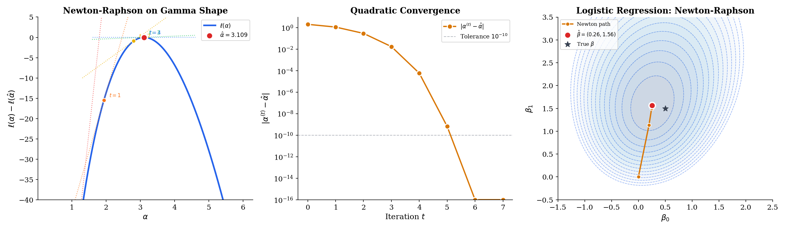
Geometrically, at each step we replace with its local quadratic approximation and jump to the maximum of that parabola. Where the log-likelihood is close to quadratic — and near the MLE it always is, by Taylor — the jump lands close to the true maximum and the next iterate does even better. This is the source of the algorithm’s speed: each iteration roughly squares the error, so -digit precision is reached in a handful of steps.
Fisher scoring is a popular variant: replace the random with its expectation , so the update becomes
For exponential families in the natural parameter, and coincide and Newton and Fisher scoring are identical. For other families, Fisher scoring often has better stability — the expected information is usually positive everywhere, while the observed information can become non-positive away from the MLE, causing Newton to take a step away from the solution.
Suppose is three times continuously differentiable in a neighborhood of the MLE , and . Then for any starting value sufficiently close to , the Newton-Raphson iterates satisfy
for some constant depending on and the third derivative of . Equivalently, the number of correct digits roughly doubles per iteration.
Proof [show]
Let denote the error at step . Taylor-expand around :
for some between and . Since is the MLE, , so
Also Taylor-expand the denominator for some between the two points. Substitute both expansions into the Newton update and subtract :
Combining the two numerator terms over the common denominator and expanding,
As , both and converge to , so the bracketed expression in the numerator approaches , and the denominator approaches . Thus, for small enough,
which is the quadratic-convergence claim.
Quadratic convergence is a very strong statement. Starting from an error of , one Newton step drops it to roughly , the next to , the next to below machine precision. In practice – iterations are enough for any likelihood that looks remotely parabolic near its maximum. This is why the “default solver” for smooth low-dimensional MLE problems is always some flavor of Newton.
For iid Gamma data with known, the log-likelihood is
Differentiate once to get the score and once more to get the Hessian:
where is the digamma function and is the trigamma function. The observed information is , so Newton-Raphson is
A standard initial guess is the method-of-moments estimate , since . From this start, convergence typically takes – iterations to machine precision. No closed-form solution exists because has no closed form — but we do not need one; Newton-Raphson handles it numerically.
Logistic regression is a binary classification model parameterized by regression coefficients on a single predictor :
Write . The Bernoulli log-likelihood, summed over iid observations,
has no closed-form maximizer — the score equations
are not linear in , since involves the sigmoid. Newton-Raphson here is the iteratively reweighted least squares (IRLS) algorithm: at each step, linearize around the current and solve a weighted linear regression with weights . In exponential-family language, IRLS is Fisher scoring; in optimization language, it is Newton-Raphson with the observed Hessian approximated by its expectation. The full GLM theory — link functions, canonical parameterizations, deviance — is developed in Topic 22 (Generalized Linear Models).
Two practical warnings: if the two classes are perfectly separable by a hyperplane (a condition called quasi-complete separation), the log-likelihood is unbounded and Newton-Raphson iterates escape to infinity — the MLE does not exist. Regularization (a ridge penalty, or a prior on ) restores finiteness — see Topic 23 §23.6 Ex 8 for the worked example on the EXAMPLE_10_GLM_DATA near-separation preset. And for neural-network-scale problems ( in the thousands to millions), computing and inverting the Hessian is infeasible; stochastic-gradient methods replace Newton-Raphson but retain its quadratic-approximation spirit when they use second-order information.
The explorer below steps through Newton-Raphson iterates on the log-likelihood. Pick a starting value with the slider, then click Step (one iteration) or Run (until convergence); the green dashed tangent at each iterate shows the slope of the score, and the next iterate is where that tangent meets zero-slope. Toggle Fisher scoring to replace with — for the Gamma-shape preset, both are and the paths coincide; for families with non-deterministic observed information they diverge.
Theorem 6 guarantees quadratic convergence once you are close enough to the MLE. Far from the MLE, three things can go wrong:
(1) Multiple local maxima. Mixture-model likelihoods have label-switching symmetries and often have multiple local maxima. Newton converges to whichever one is closest; standard practice is to run EM or Newton from many random starting points and keep the best.
(2) Saddle points. In higher dimensions, the Hessian can have mixed signs away from the MLE. Newton-Raphson at a saddle point takes a “step” that increases in some directions and decreases in others — the iteration can stall or oscillate. Fisher scoring, by using the expected (positive-definite) information, avoids this pathology.
(3) Diverging iterates. If the starting point is in a region where the log-likelihood is flat or inverted in curvature, the Newton step can overshoot wildly. Line search (backtracking until actually increases) is the standard safeguard — guaranteed convergence at the cost of sometimes making small steps.
For the low-dimensional, smooth, exponential-family MLEs that dominate classical statistics, none of this is a concern: start anywhere reasonable, and Newton finds the MLE in – steps. The pathologies become important precisely at the frontier between classical statistics and modern ML — which is where non-convex likelihoods, high dimensions, and exotic parameterizations live.
14.8 Observed and Expected Fisher Information
The asymptotic-normality theorem uses the expected Fisher information — a deterministic function of the unknown parameter. In practice, we estimate the asymptotic variance from data, which forces a choice: plug in into the expected information, or use the observed (data-dependent) information? Both are consistent; both appear in textbooks and software; but they are not identical, and the choice matters.
The observed Fisher information at is the negative Hessian of the log-likelihood:
It is a random variable (depends on the sample) and is typically evaluated at the MLE: .
The distinction from the expected information is purely one of averaging. The expected information is a deterministic function of ; it is what you would compute if you could integrate against the true density. The observed information is what you get when you sum over the actual data you have — the sample analog. By the LLN, , so they agree in the limit; at any finite they differ by .
Under the conditions of Theorem 4,
The first statement is the LLN applied to the iid sequence . The second extends this by continuous mapping plus the consistency of from Theorem 3. Both information quantities, evaluated at the MLE, are consistent estimators of — so either can be used to construct a Wald confidence interval
Both are asymptotically valid. The practical question is: which one produces better coverage at finite ?
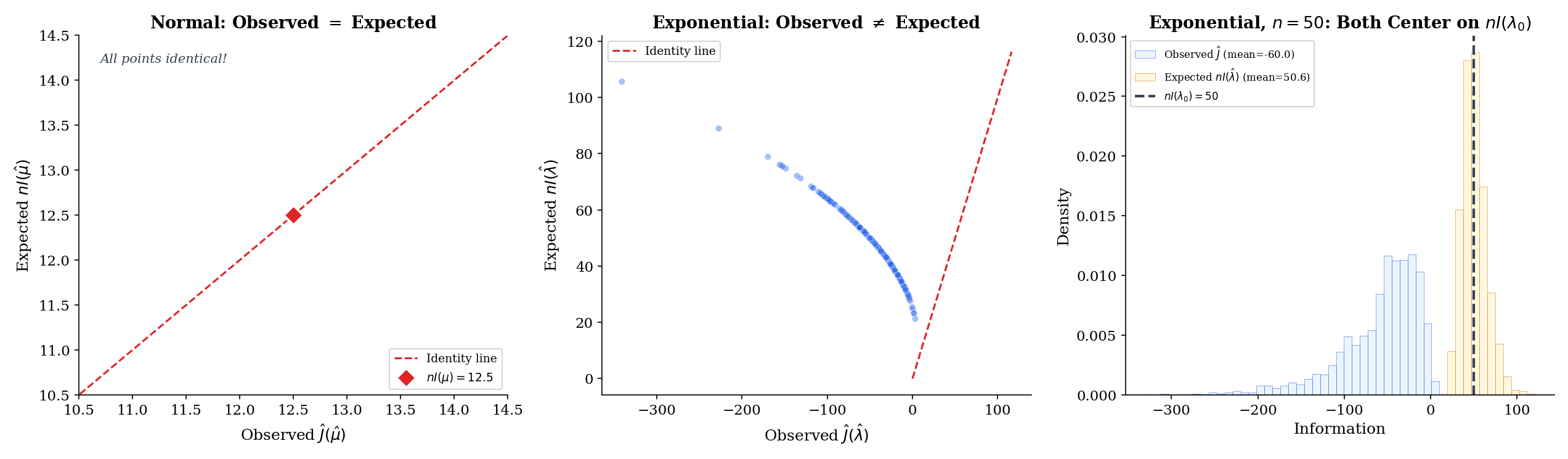
For Normal data with known, , independent of . Therefore
The observed information equals times the expected information exactly at every and for every sample — there is no randomness in . This is the “no-surprises” case and makes the Normal-mean Wald interval unambiguous: the two constructions agree at every sample.
For Exponential, , again independent of , so
Evaluated at the MLE ,
So observed and expected information, evaluated at the MLE, coincide identically — but both are now random, varying sample-to-sample through . The same is true of Bernoulli and Poisson at the MLE: in each exponential-family case, the score equation makes the Hessian lose its data-dependence at the MLE, so observed and expected information become equal there. This is a property of exponential families in the natural parameter, not a universal one; for Cauchy location, say, observed and expected information at the MLE differ in finite samples. The below visualizes the sample-to-sample variation of around the deterministic anchor .
The Monte-Carlo explorer below realizes both and across 200 replicates. Notice the qualitative difference between the Normal-mean preset — where the scatter collapses to a single point at — and the Exponential / Poisson / Bernoulli presets, where the scatter is on the identity line but spreads along it as varies. As grows, the cloud contracts toward the deterministic anchor , visualized as an open black circle.
In a classic paper, Bradley Efron and David Hinkley argued that the observed information is generally preferable to the expected information for constructing confidence intervals — even when the MLE sits at a point where the two agree identically. The reason is that conditions on the sample, capturing the sample-specific curvature of the log-likelihood at the observed data. When the sample happens to be highly informative (curvature steep), reflects that and gives a narrower interval; when the sample is less informative (curvature shallow), gives a wider one — both calibrated to what the data actually tell you.
For exponential families the two quantities agree at the MLE (Example 16), so there is no practical distinction. For non-exponential families, the Efron–Hinkley result says “use .” This is the default in most modern software: in R reports standard errors based on the observed information, not the expected information, unless you explicitly ask otherwise.
The broader lesson is that all consistency-level statements (Theorem 7) let you swap for asymptotically, but finite-sample calibration can favor one or the other. In Bayesian language, this parallels the difference between posterior variance and prior-predictive variance — both are “variance”, but they answer different questions.
14.9 Connections to Machine Learning
Every ML practitioner uses maximum likelihood daily, often without calling it that. The three most important translations are cross-entropy, MAP/regularization, and the exponential-family MLE recipe — and they are all re-readings of §§14.1–14.8 in ML notation.
Suppose is a categorical outcome with class probabilities depending on a parameter (e.g., via a softmax layer in a neural network). The log-likelihood for one observation is , and summed over the training set,
The inner sum over is the cross-entropy between the one-hot empirical distribution at observation and the model distribution . Summing over and dividing by gives the mean cross-entropy. So “minimize cross-entropy loss” and “maximize Bernoulli/categorical log-likelihood” are literally the same objective up to a sign and a constant.
When the model is a neural network with a softmax output, the score equation is the vanishing-gradient condition backpropagation computes. Every gradient descent step in a classification training loop is a (stochastic, approximate) step toward the MLE of a categorical likelihood. Every well-trained classifier is an approximate MLE.
For any exponential family written in canonical form , Topic 7 §7.8 derived the universal MLE recipe:
In words: the MLE of the natural parameter is the value at which the expected sufficient statistic under the model equals the sample average of the sufficient statistic. This is the most compact statement of MLE for a single parametric family — it covers all nine of the classical exponential-family examples (Normal, Bernoulli, Poisson, Gamma, Beta, and their relatives) in one formula.
For a single-predictor logistic regression, the natural parameter is , the sufficient statistic is , and . The MLE equation becomes at each -value — the fitted probabilities match the empirical fractions. For a Poisson regression with log-link, and ; the MLE equation becomes per covariate level. The entire “exponential-family GLM” pipeline — logistic, Poisson, linear, gamma, and beyond — is moment matching on the sufficient statistics.
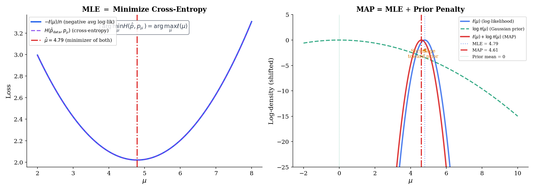
Every Bayesian posterior has the form , where is the prior. Taking logs,
The maximum-a-posteriori (MAP) estimate is the maximizer of this log-posterior — equivalently, the maximizer of . Compared to the MLE, MAP adds the log-prior as a penalty term. Two canonical examples light up immediately:
Gaussian prior: gives
which is the / ridge / weight-decay penalty. Laplace prior: gives
which is the / lasso / sparsity penalty.
Ridge regression is MAP estimation with a Gaussian prior on the coefficients; lasso is MAP estimation with a Laplace prior (Topic 23 §23.7 Thm 5 formalizes this correspondence). Weight decay in a neural network is MAP with a Gaussian prior on the weights. The regularization parameter — in the Gaussian case, in the Laplace case — is a prior hyperparameter, which can in turn be learned by empirical Bayes or set by cross-validation. The Bernstein–von Mises theorem says that under regularity, the posterior concentrates around the MLE at rate in total variation: priors stop mattering once there is enough data. Topic 25 §25.8 develops this with a sketch proof following van der Vaart 1998 §10. The “Bayesian bridge” is exactly this: regularization is a prior, and the prior is informative only until the data overwhelm it.
This is why every modern ML optimizer — Adam, AdamW, L-BFGS with L² regularization — can be read as a MAP procedure. The loss is the negative log-likelihood; the weight-decay term is the negative log-prior; the minimum is the MAP estimate. When someone asks “is neural-network training frequentist or Bayesian?” the honest answer is: it is MAP, which is both at once, and the amount of regularization decides which side dominates.
14.10 Summary
The maximum-likelihood estimator ties together everything in Topics 1–13 — likelihoods come from the densities of Topics 5–6; the score and Fisher information come from Topic 13; consistency comes from Topic 10’s law of large numbers; asymptotic normality comes from Topic 11’s central limit theorem together with Topic 9’s Slutsky theorem; efficiency comes from Topic 13’s Cramér-Rao lower bound. The result is a single procedure that is consistent, asymptotically normal, and asymptotically efficient under regularity — no other estimator in the regular class beats it in the limit.
| Property | Statement | Ingredients |
|---|---|---|
| Existence (interior MLE) | Score equation has a solution | open, differentiable |
| Invariance | Change of variables or profile likelihood | |
| Consistency | Compact , KL-identifiable, LLN + Gibbs inequality | |
| Asymptotic normality | Taylor + CLT + LLN + Slutsky | |
| Asymptotic efficiency | CRLB | Theorem 4 + Theorem 9 of Topic 13 |
| Computation | Newton-Raphson: | Quadratic convergence near MLE |
Cheat sheet for the four workhorse families:
| Family | Parameter | MLE | Fisher info | CRLB | Wald 95% CI |
|---|---|---|---|---|---|
| Normal | (σ² known) | ||||
| Bernoulli | |||||
| Exponential | |||||
| Poisson |
Where this leads. Method of Moments applies the Topic 13 framework to moment-matching estimators, comparing their efficiency to the MLE benchmark developed here — asymptotic relative efficiency ARE(MoM, MLE) is typically for families outside the natural exponential representation. Sufficient Statistics uses Fisher information and the CRLB to prove Rao–Blackwell and Lehmann–Scheffé, showing that the MLE is always a function of the sufficient statistic when one exists. Hypothesis Testing (Topic 17) introduces the likelihood-ratio test, the Wald test, and the score test as a trio of asymptotically tests, all corollaries of Thm 14.3 via Slutsky and continuous mapping. The full proof of Wilks’ is Topic 18’s territory; Topic 17 states the result and derives the Wald case in a two-line application of asymptotic normality. Confidence Intervals constructs Wald, score, and profile intervals all from the landscape. Generalized Linear Models lifts logistic regression to its full glory: MLE for exponential-family outcomes with link functions, solved by iteratively-reweighted least squares — which is Newton-Raphson/Fisher scoring from §14.7. And Bayesian Foundations formalizes the MAP/regularized-MLE correspondence of Remark 9, giving a principled framework for the informative priors that regularization has been quietly deploying. §25.8 Ex 8 closes the arc from Topic 14 §14.11 Rem 9 through Topic 23 §23.7 Thm 5.
Across formalML, maximum likelihood organizes almost everything: the training objective of a classifier is a Bernoulli/categorical log-likelihood; the training objective of a regressor is a Gaussian log-likelihood; the training of a variational autoencoder is an ELBO — a lower bound on a likelihood — optimized by gradient ascent. The reader who has understood this topic has understood the statistical backbone of modern machine learning. Every optimizer, every loss function, every regularization penalty is a paragraph of §§14.1–14.9 written in a different notation.
Appendix: The EM Algorithm
Some log-likelihoods are intractable not because is big but because the model has latent variables. The canonical example is a Gaussian mixture: each observation comes from one of Gaussians, but we do not observe which. Write for the unobserved mixture component and for the parameters. The marginal density of is
where is the Normal density. The log-likelihood has the logarithm of a sum, which does not simplify and has no closed-form maximizer.
The expectation-maximization (EM) algorithm side-steps this by alternating between two simpler problems. At the current parameter estimate :
- E-step. Compute the posterior probabilities — the “responsibility” of component for observation .
- M-step. Maximize the expected complete-data log-likelihood: . This decouples into a weighted Normal MLE for each component, which is just weighted sample means and weighted sample variances — closed-form.
Each EM iteration increases the log-likelihood: , with equality only at a stationary point. The EM algorithm converges to a local maximum of ; the global maximum in a mixture model usually requires multiple random restarts, since the likelihood surface is highly multimodal. The full theory — Jensen’s inequality applied to the log, the ELBO lower bound, convergence rates and monotonicity — is developed in Bayesian Foundations (Topic 25) and formalml’s formalML: Variational Methods . For this topic, EM is the right tool when the MLE is defined but hard to compute directly, and factors cleanly once the latent variable is conditioned on.
References
- Casella, G., & Berger, R. L. (2002). Statistical Inference (2nd ed.). Duxbury.
- Lehmann, E. L., & Casella, G. (1998). Theory of Point Estimation (2nd ed.). Springer.
- van der Vaart, A. W. (1998). Asymptotic Statistics. Cambridge University Press.
- Wasserman, L. (2004). All of Statistics. Springer.
- Bickel, P. J., & Doksum, K. A. (2015). Mathematical Statistics: Basic Ideas and Selected Topics (2nd ed.). CRC Press.
- Bishop, C. M. (2006). Pattern Recognition and Machine Learning. Springer.
- Nocedal, J., & Wright, S. J. (2006). Numerical Optimization (2nd ed.). Springer.