Uniform, Normal, Exponential, Gamma, Beta, Chi-squared, Student's t, and F — the named PDFs that underpin statistical inference and machine learning, each derived from a distinct probabilistic mechanism.
Topic 5 — Discrete Distributions cataloged seven discrete PMFs. We now turn to the continuous side: eight distributions, each arising from a distinct probabilistic mechanism, each receiving the same systematic treatment — PDF, moments, MGF, key property, ML connection.
The difference is calculus, not philosophy. Where the discrete catalog summed PMFs, this one integrates PDFs. The tools we built in Expectation, Variance & Moments — E[X]=∫xf(x)dx, Var(X)=E[X2]−(E[X])2, MGFs — carry over directly. What changes is the palette: these distributions live on continuous supports, their densities are smooth curves, and their moments require the integration techniques from formalCalculus: .
Remark 1 A Parallel Catalog
This topic mirrors Discrete Distributions by design. Five core distributions (Uniform, Normal, Exponential, Gamma, Beta) are independently motivated with full derivations. Three derived distributions (Chi-squared, Student’s t, F) are defined by construction from the Normal and Chi-squared. The core five receive the same template as Topic 5: definition, then E[X] and Var(X) proofs, then MGF, then key properties, then an ML connection. The derived three share a single section — they are building blocks for hypothesis testing rather than independent modeling choices.
The interactive explorer below lets you switch between all eight distributions, adjust their parameters, and see how the PDF, CDF, and moments respond.
Interactive: Continuous Distribution Catalog Explorer
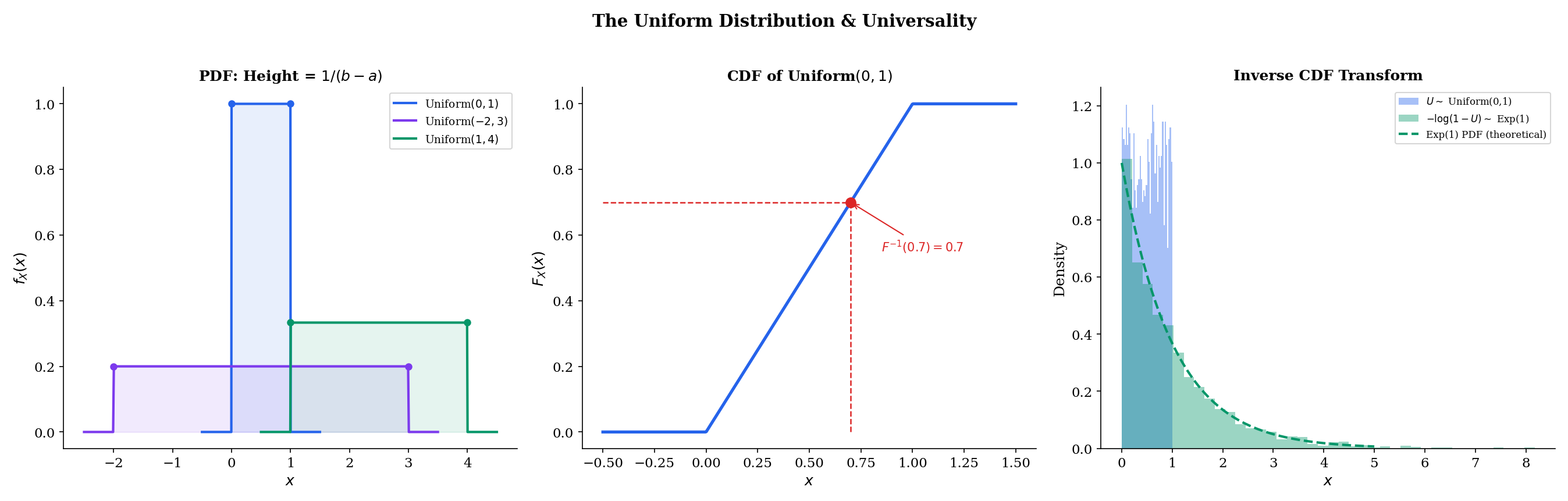
The Uniform distribution is the continuous version of maximum ignorance: every point in an interval is equally likely. It is the simplest continuous distribution and the starting point for simulation — we can transform Uniform samples into samples from any other distribution via the inverse CDF method.
Definition 1 Continuous Uniform Distribution
A random variable X has the Uniform distribution on [a,b], written X∼Uniform(a,b), if its PDF is
f(x)={b−a10if a≤x≤b,otherwise.
The CDF is F(x)=b−ax−a for x∈[a,b], with F(x)=0 for x<a and F(x)=1 for x>b.
The PDF is flat — constant density over the interval, zero outside. The normalization condition ∫abb−a1dx=1 is immediate.
Remark 2 The Uniform Is NOT an Exponential Family Member
Unlike the other four core distributions in this topic, the Uniform is not a member of the exponential family. The reason: its support [a,b] depends on the parameters. The exponential family requires that the support of the density be independent of the parameters — a condition the Uniform violates. Exponential Families makes this distinction precise.
Example 1 Inverse CDF Transform: Generating Exponential Samples
If U∼Uniform(0,1) and we define X=F−1(U)=−λ1ln(1−U), then X∼Exponential(λ). This is the inverse CDF transform — a fundamental simulation technique.
Proof.P(X≤x)=P(−λ1ln(1−U)≤x)=P(U≤1−e−λx)=1−e−λx, which is the Exponential CDF. Since 1−U has the same distribution as U, we can simplify to X=−λ1lnU.
ML connection. Every random number generator starts with Uniform samples. The inverse CDF transform converts them to any target distribution — as long as F−1 can be computed. For the Normal, Φ−1 has no closed form, so specialized algorithms (Box-Muller, Ziggurat) are used instead.
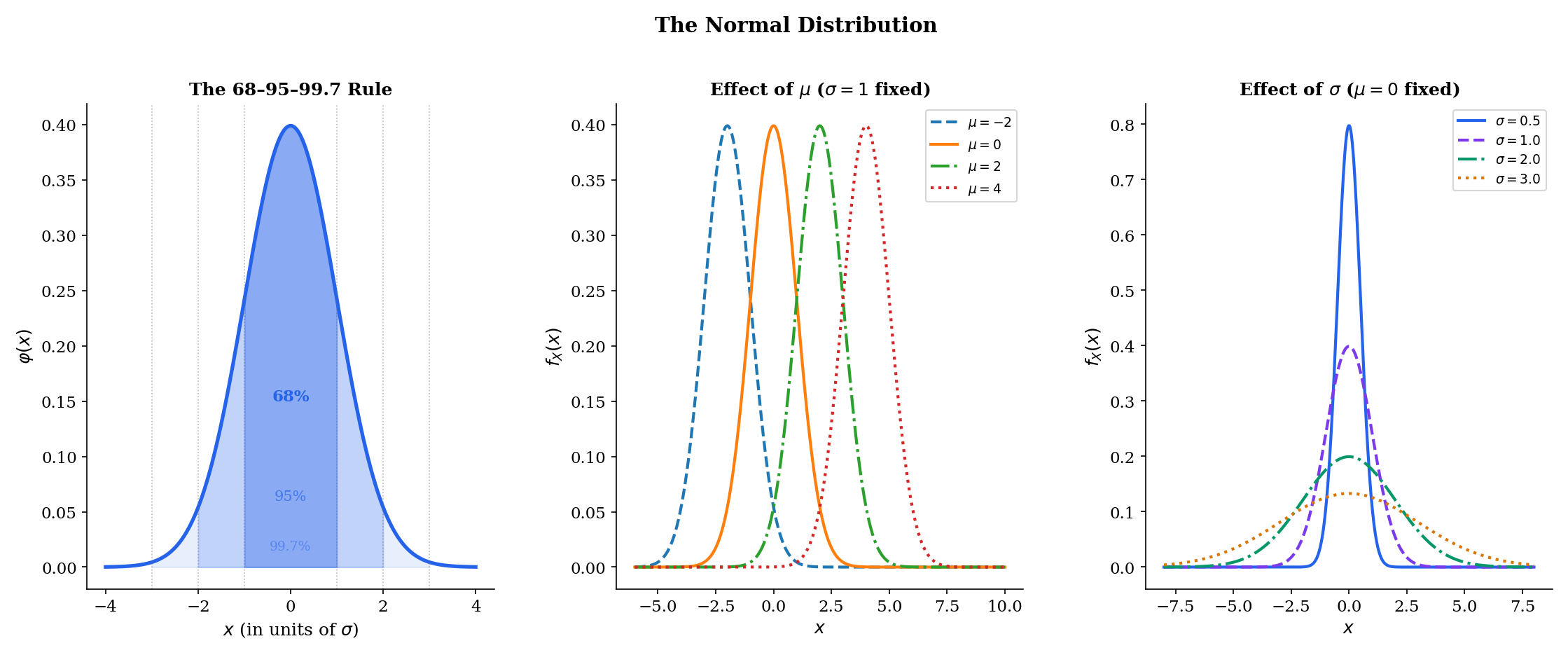
6.3 The Normal Distribution
The Normal distribution is the most important distribution in all of statistics. Its centrality comes from the Central Limit Theorem: sums of many independent random variables converge to Normal form, regardless of the original distribution. This makes the Normal the universal approximation for aggregate effects — measurement errors, test scores, stock returns over short intervals, and noise in machine learning models.
Definition 2 Normal Distribution
A random variable X has the Normal distribution with mean μ and variance σ2, written X∼N(μ,σ2), if its PDF is
f(x)=σ2π1exp(−2σ2(x−μ)2),x∈R
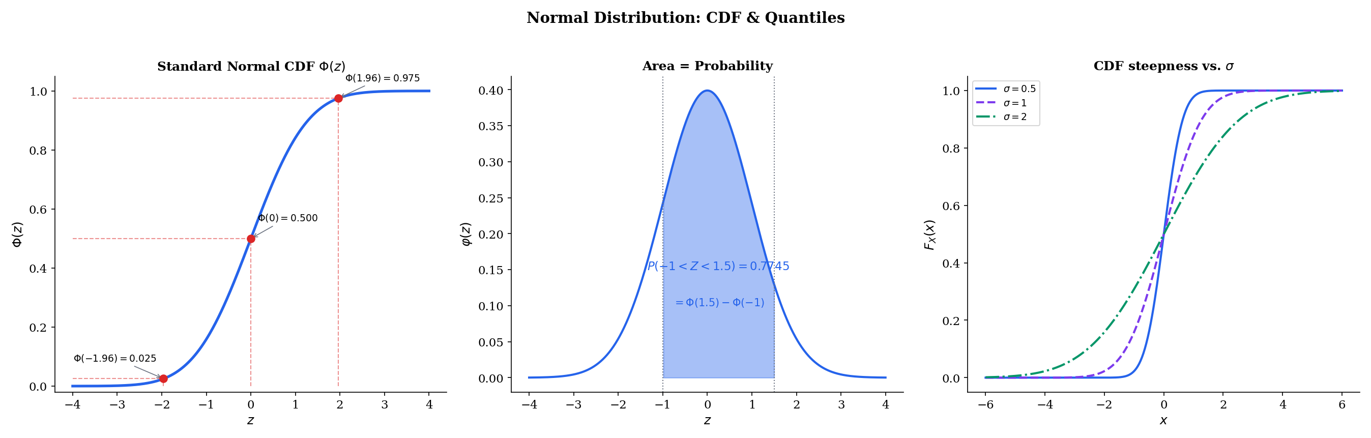
The special case Z∼N(0,1) is the standard Normal, with PDF φ(z)=2π1e−z2/2 and CDF Φ(z)=∫−∞zφ(t)dt.
The PDF is the familiar bell curve, symmetric about μ. That ∫−∞∞e−z2/2dz=2π — the Gaussian integral — is a classical result from formalCalculus: .
Theorem 2 Normal Moments
If X∼N(μ,σ2), then E[X]=μ and Var(X)=σ2.
Proof
[show][hide]
Expectation. Standardize: let Z=(X−μ)/σ, so X=μ+σZ where Z∼N(0,1).
E[X]=E[μ+σZ]=μ+σE[Z]
Now E[Z]=∫−∞∞z⋅φ(z)dz=0 by the symmetry of φ about zero (the integrand ze−z2/2 is an odd function). So E[X]=μ.
Variance.Var(X)=σ2Var(Z), so it suffices to show Var(Z)=E[Z2]=1. We compute:
E[Z2]=∫−∞∞z2⋅2π1e−z2/2dz
Integrate by parts with u=z and dv=ze−z2/2dz, giving v=−e−z2/2:
E[Z2]=2π1[−ze−z2/2]−∞∞+2π1∫−∞∞e−z2/2dz
The boundary term vanishes (the exponential kills the polynomial). The remaining integral is 2π, so E[Z2]=2π2π=1.
Therefore Var(X)=σ2⋅1=σ2.
□
◼
Theorem 3 Normal MGF
If X∼N(μ,σ2), then MX(t)=exp(μt+2σ2t2) for all t∈R.
Proof
[show][hide]
We compute directly, using the completing-the-square technique from formalCalculus: :
MX(t)=E[etX]=∫−∞∞etx⋅σ2π1exp(−2σ2(x−μ)2)dx
Combine the exponents: tx−2σ2(x−μ)2. Complete the square in x:
This is the MGF of N(μ1+μ2,σ12+σ22). Since MGFs uniquely determine distributions, X1+X2∼N(μ1+μ2,σ12+σ22).
□
◼
The Normal is closed under addition of independent variables. This is the reproductive property — and it is the algebraic reason the Normal appears everywhere. Any sum of independent Normal variables is still Normal.
Theorem 5 Normal Linear Transformation
If X∼N(μ,σ2) and a,b are constants with a=0, then aX+b∼N(aμ+b,a2σ2).
In particular, the standardizationZ=(X−μ)/σ∼N(0,1) is a special case with a=1/σ and b=−μ/σ.
Remark 3 Normal Exponential Family Form
The Normal belongs to the exponential family with natural parameters η1=μ/σ2 and η2=−1/(2σ2). The sufficient statistics are (X,X2). When σ2 is known, the single natural parameter η=μ/σ2 makes MLE particularly clean: the sufficient statistic is Xˉ, and the MLE is μ^=Xˉ. Exponential Families develops this systematically.
Interactive: Normal Properties Explorer
μ ± 1σ: 68.27%μ ± 2σ: 95.45%μ ± 3σ: 99.73%
Example 2 Normal MLE: Why Minimizing Squared Error Is MLE Under Gaussian Noise
Suppose we observe data y1,…,yn and model yi=f(xi)+εi where εi∼N(0,σ2) independently. The log-likelihood is:
ℓ(θ)=−2nln(2πσ2)−2σ21i=1∑n(yi−f(xi))2
Maximizing ℓ(θ) with respect to θ (the parameters of f) is equivalent to minimizing ∑i=1n(yi−f(xi))2. This is why least squares = MLE under Gaussian noise. The assumption of Normal errors is baked into every ordinary least squares regression — and when that assumption fails, the MLE changes (e.g., to Laplace errors for ℓ1 loss). See Topic 22 (Generalized Linear Models) for the general framework.
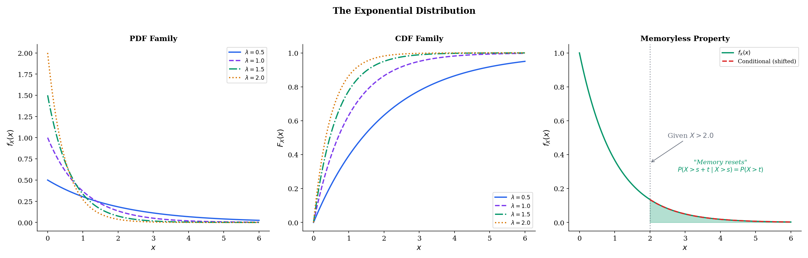
6.4 The Exponential Distribution
The Exponential distribution models waiting times in a Poisson process: if events arrive at a constant rate λ, the time between consecutive events is Exponential(λ). Its defining property is memorylessness — the time already waited provides no information about the remaining wait.
Definition 3 Exponential Distribution
A random variable X has the Exponential distribution with rate λ>0, written X∼Exponential(λ), if its PDF is
f(x)=λe−λx,x≥0
The CDF is F(x)=1−e−λx for x≥0. The mean is 1/λ and the median is ln2/λ.
Theorem 6 Exponential Moments
If X∼Exponential(λ), then E[X]=λ1 and Var(X)=λ21.
For t≥λ, the integral diverges, so the MGF is defined only for t<λ.
□
◼
Theorem 8 Exponential Memoryless Property
A continuous random variable X with support [0,∞) satisfies the memoryless property P(X>s+t∣X>s)=P(X>t) for all s,t≥0 if and only if X∼Exponential(λ) for some λ>0.
Proof
[show][hide]
Forward direction. Suppose X∼Exponential(λ). Then P(X>x)=e−λx for x≥0. By the definition of conditional probability:
Reverse direction. Suppose P(X>s+t∣X>s)=P(X>t) for all s,t≥0. Let g(x)=P(X>x). Then g(s+t)=g(s)⋅g(t) for all s,t≥0. This is Cauchy’s functional equation on [0,∞). Under the mild regularity condition that g is monotone (which follows from g being a survival function), the only solution is g(x)=e−λx for some λ>0. This gives F(x)=1−e−λx, which is the Exponential CDF.
□
◼
The memoryless property has a vivid interpretation: if you’ve been waiting 10 minutes for a bus with Exponential interarrival times, the conditional distribution of additional wait time is the same as if you’d just arrived. The past provides no information about the future. This is the continuous analog of the Geometric memoryless property from Discrete Distributions.
Remark 4 Exponential Exponential Family Form
The Exponential belongs to the exponential family with natural parameter η=−λ and sufficient statistic T(x)=x. The log-partition function is A(η)=−ln(−η), and E[X]=A′(η)=1/λ. Exponential Families shows how this structure enables conjugate Bayesian inference: the Gamma distribution is the conjugate prior for the Exponential rate parameter.
The waiting time "resets" — the past provides no information about the remaining time.
Example 3 Exponential Survival Analysis: Constant Hazard
In survival analysis, the hazard functionh(t)=f(t)/(1−F(t)) measures the instantaneous failure rate at time t, given survival to t. For the Exponential:
h(t)=e−λtλe−λt=λ
The hazard is constant — the system does not age. This makes the Exponential a baseline model: real systems wear out (h(t) increasing, Weibull distribution) or burn in (h(t) decreasing). Departures from constant hazard motivate the Gamma and Weibull alternatives. In ML, Exponential survival models appear in customer churn prediction, equipment failure forecasting, and time-to-event modeling.
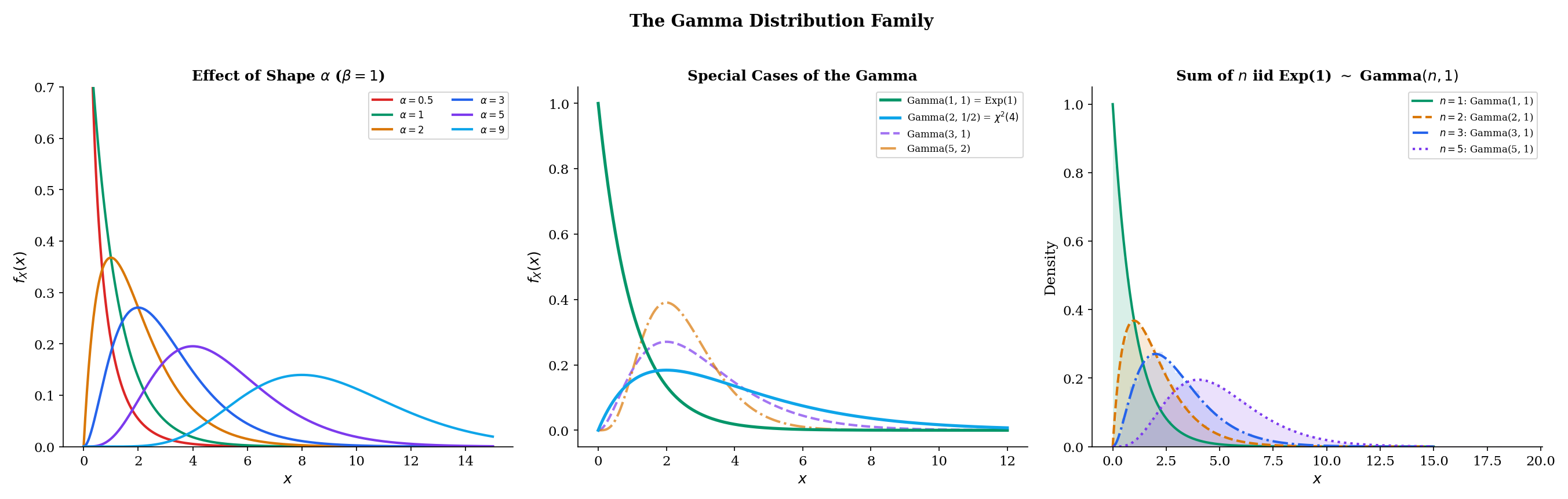
6.5 The Gamma Distribution
The Gamma distribution generalizes the Exponential in a natural way: if the Exponential models the time until the first event in a Poisson process, the Gamma models the time until the α-th event. It subsumes the Exponential (α=1) and the Chi-squared (α=k/2, β=1/2) as special cases.
Before defining the Gamma distribution, we need the Gamma function — the normalization constant that makes the PDF integrate to 1.
Recursion:Γ(α+1)=αΓ(α). This follows from formalCalculus: : with u=tα and dv=e−tdt, the boundary terms vanish and we get Γ(α+1)=α∫0∞tα−1e−tdt=αΓ(α).
Factorial connection: Since Γ(1)=∫0∞e−tdt=1, the recursion gives Γ(n)=(n−1)! for every positive integer n. The Gamma function extends the factorial to non-integer arguments.
Half-integer value:Γ(1/2)=π. This follows from the substitution t=u2/2, which converts Γ(1/2) into the Gaussian integral ∫−∞∞e−u2/2du=2π.
Definition 4 Gamma Distribution
A random variable X has the Gamma distribution with shape α>0 and rate β>0, written X∼Gamma(α,β), if its PDF is
f(x)=Γ(α)βαxα−1e−βx,x>0
The normalization follows from the Gamma function: the substitution u=βx transforms ∫0∞Γ(α)βαxα−1e−βxdx into Γ(α)1∫0∞uα−1e−udu=1.
Theorem 9 Gamma Moments
If X∼Gamma(α,β), then E[X]=βα and Var(X)=β2α.
Proof
[show][hide]
Expectation. We compute directly, using the Gamma function recursion:
If X1∼Gamma(α1,β) and X2∼Gamma(α2,β) are independent (with the same rateβ), then
X1+X2∼Gamma(α1+α2,β)
Proof
[show][hide]
By MGFs:
MX1+X2(t)=(β−tβ)α1⋅(β−tβ)α2=(β−tβ)α1+α2
This is the MGF of Gamma(α1+α2,β).
□
◼
In particular, if X1,…,Xn∼Exponential(β) are independent, then X1+⋯+Xn∼Gamma(n,β). This confirms the Poisson process interpretation: the sum of n independent Exponential waiting times has a Gamma distribution.
Remark 6 Gamma Exponential Family Form
The Gamma belongs to the exponential family with natural parameters η1=α−1 and η2=−β, and sufficient statistics (X,lnX). When α is known, the single natural parameter is η=−β with sufficient statistic T(x)=x, and the conjugate prior for β is itself a Gamma. Exponential Families unifies this with the Exponential’s exponential family form.
Insurance claim amounts are positive and right-skewed — large claims are rare but impactful. The Gamma distribution is a natural model: the shape parameter α controls the skewness, and the rate β controls the scale. In a Gamma GLM, we model claim amounts Yi∼Gamma(α,βi) with lnE[Yi]=β0+β1xi1+⋯ (log link), allowing covariates (driver age, vehicle type, region) to affect the expected claim size while maintaining the Gamma’s positive support and right skew. See Topic 22 §22.6 (Gamma regression) for the full GLM framework and the worked insurance-amounts example.
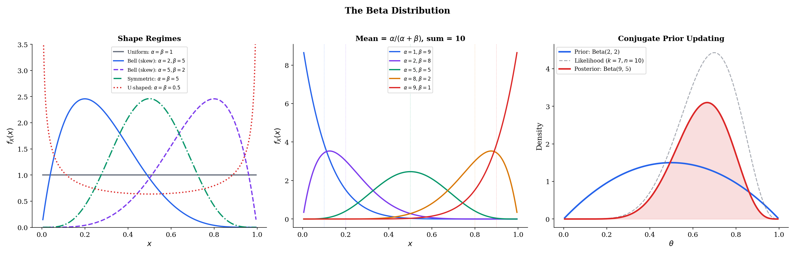
6.6 The Beta Distribution
The Beta distribution lives on [0,1] — precisely the range of a probability parameter. This makes it the natural distribution for modeling uncertainty about unknown probabilities, success rates, and proportions. Its two shape parameters give it remarkable flexibility: it can be uniform, bell-shaped, U-shaped, J-shaped, or heavily skewed.
Definition 5 Beta Distribution
A random variable X has the Beta distribution with parameters α>0 and β>0, written X∼Beta(α,β), if its PDF is
f(x)=Γ(α)Γ(β)Γ(α+β)xα−1(1−x)β−1,0<x<1
The normalizing constant B(α,β)=Γ(α+β)Γ(α)Γ(β) is the Beta function.
The mean E[X]=α/(α+β) has a beautiful interpretation: α is the “number of successes” and β is the “number of failures” in the prior’s pseudo-data. As we collect real data, α and β grow, and the distribution concentrates around the true probability.
Theorem 13 Beta-Bernoulli Conjugacy
If the prior on θ is Beta(α,β) and we observe k successes in n independent Bernoulli(θ) trials, then the posterior is
θ∣data∼Beta(α+k,β+n−k)
Proof
[show][hide]
By Bayes’ theorem, the posterior is proportional to the prior times the likelihood:
p(θ∣k)∝p(k∣θ)⋅p(θ)
The Binomial likelihood is p(k∣θ)∝θk(1−θ)n−k. The Beta prior is p(θ)∝θα−1(1−θ)β−1. Multiplying:
This is the kernel of a Beta(α+k,β+n−k) density. Since the posterior must integrate to 1, the normalizing constant is B(α+k,β+n−k).
□
◼
This is conjugacy: the prior and posterior belong to the same family. The update rule is additive: add k to α (successes) and n−k to β (failures). The posterior mean is:
E[θ∣k]=α+β+nα+k
This is a weighted average of the prior mean α/(α+β) and the sample proportion k/n, with weights proportional to the “sample sizes” α+β (prior) and n (data). As n→∞, the posterior concentrates around the true θ regardless of the prior — the data overwhelms prior beliefs.
Remark 7 Beta Exponential Family Form
The Beta belongs to the exponential family with natural parameters η1=α−1 and η2=β−1, and sufficient statistics (lnX,ln(1−X)). The log-partition function is A(η1,η2)=lnΓ(η1+1)+lnΓ(η2+1)−lnΓ(η1+η2+2). Exponential Families connects this to the Beta-Bernoulli conjugacy via the general theory of conjugate priors.
Interactive: Beta-Bernoulli Conjugate Prior
— Prior Beta(1.0, 1.0)— Posterior Beta(8.0, 14.0)
Prior
E[θ] = 0.5000
95% CI: [0.025, 0.975]
Eff. sample size: 2.0
Posterior
E[θ|data] = 0.3636
95% CI: [0.181, 0.570]
Eff. sample size: 22.0
As n → ∞, the posterior concentrates around the true θ regardless of the prior.
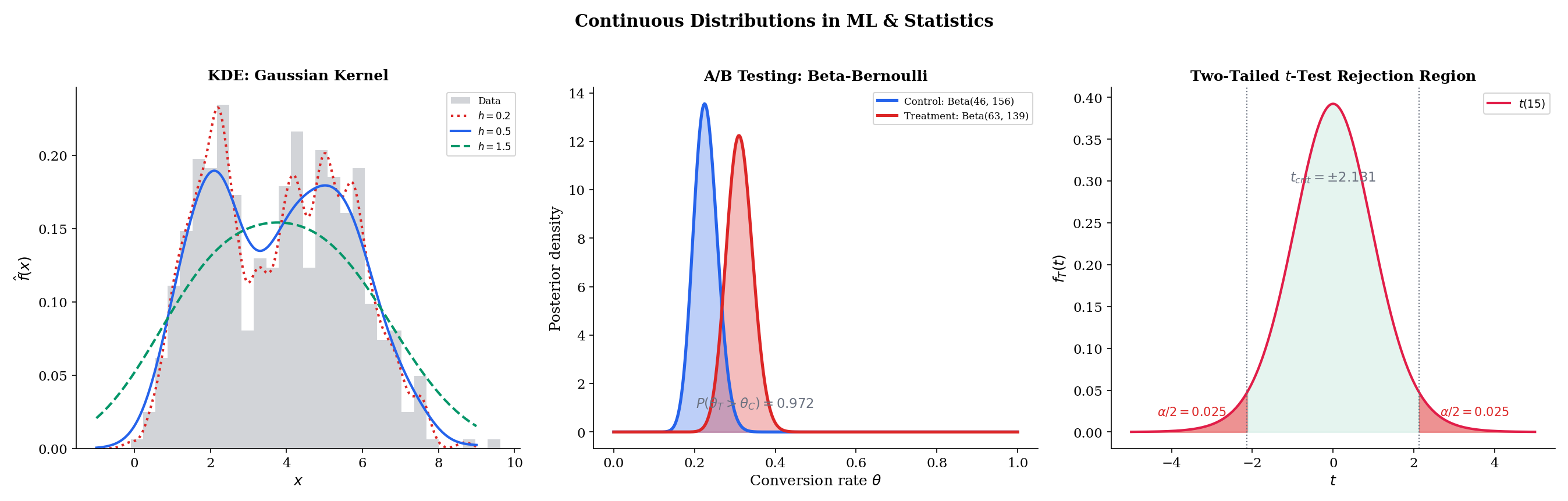
Example 5 Beta-Bernoulli A/B Testing
A company runs an A/B test comparing two button designs. Design A has a Beta(1,1) prior (uniform — no prior information about the click rate). After 200 users see Design A, 34 click. The posterior is Beta(1+34,1+166)=Beta(35,167).
The posterior mean click rate is 35/202≈0.173, with a 95% credible interval of approximately [0.124,0.231].
Design B, with prior Beta(1,1) and 42 clicks from 200 users, has posterior Beta(43,159), mean 43/202≈0.213.
The probability that Design B is better, P(θB>θA∣data), can be computed by Monte Carlo: draw from each posterior, count how often θB>θA. This is Bayesian A/B testing — and it starts with the Beta-Bernoulli conjugate pair. Bayesian Foundations (Topic 25) develops the general framework, including the posterior predictive for the Beta-Binomial compound.
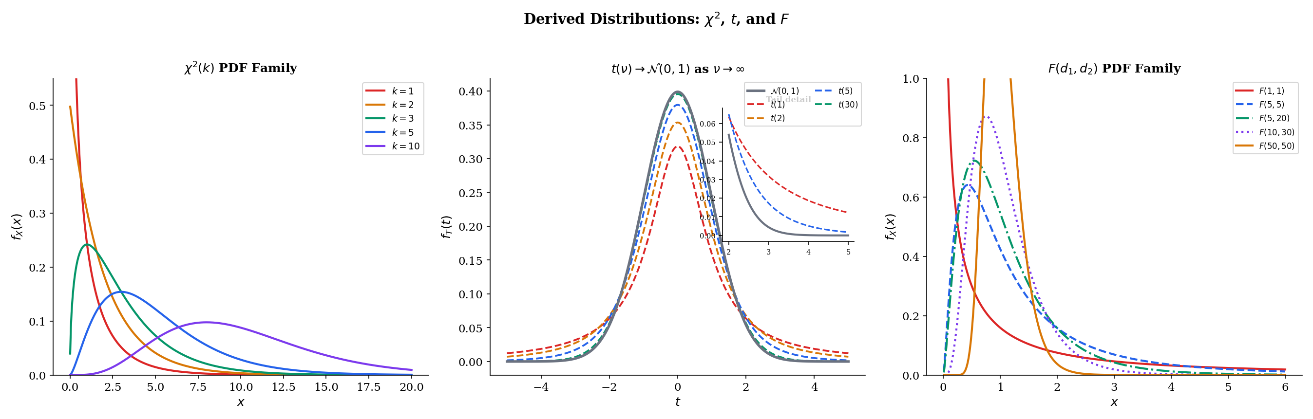
6.7 Derived Distributions: Chi-squared, Student’s t, and F
The next three distributions are not independently motivated by a random mechanism. Instead, they are derived from the Normal distribution through specific constructions. They form the test statistic distributions for classical hypothesis testing.
Definition 6 Chi-squared Distribution
If Z1,…,Zk are independent N(0,1) random variables, then
X=Z12+Z22+⋯+Zk2∼χ2(k)
has the Chi-squared distribution with k degrees of freedom. Equivalently, χ2(k)=Gamma(k/2,1/2).
The equivalence with Gamma(k/2,1/2) follows because Z2∼Gamma(1/2,1/2) (proved via the formalCalculus: formula), and the Gamma reproductive property gives Z12+⋯+Zk2∼Gamma(k/2,1/2).
Theorem 14 Chi-squared Moments
If X∼χ2(k), then E[X]=k and Var(X)=2k.
Proof
[show][hide]
Since χ2(k)=Gamma(k/2,1/2), we apply the Gamma moment formulas:
E[X]=βα=1/2k/2=kVar(X)=β2α=1/4k/2=2k
□
◼
Theorem 15 Chi-squared MGF
If X∼χ2(k), then MX(t)=(1−2t)−k/2 for t<1/2.
Proof
[show][hide]
From the Gamma MGF with α=k/2 and β=1/2:
MX(t)=(1/2−t1/2)k/2=(1−2t1)k/2=(1−2t)−k/2
□
◼
Theorem 16 Chi-squared Reproductive Property
If X1∼χ2(k1) and X2∼χ2(k2) are independent, then X1+X2∼χ2(k1+k2).
Proof
[show][hide]
This is the Gamma reproductive property with β=1/2:
Alternatively, by MGFs: (1−2t)−k1/2⋅(1−2t)−k2/2=(1−2t)−(k1+k2)/2.
□
◼
Definition 7 Student's t Distribution
If Z∼N(0,1) and V∼χ2(ν) are independent, then
T=V/νZ∼t(ν)
has Student’s t distribution with ν degrees of freedom. Its PDF is:
f(t)=νπΓ(2ν)Γ(2ν+1)(1+νt2)−(ν+1)/2,t∈R
The t distribution looks like a Normal but has heavier tails — extreme values are more likely. As ν increases, the tails thin and the t converges to the standard Normal.
Theorem 17 Student's t Moments
If T∼t(ν), then:
E[T]=0 for ν>1 (undefined for ν≤1)
Var(T)=ν−2ν for ν>2 (infinite for 1<ν≤2, undefined for ν≤1)
Proof
[show][hide]
Part 1. The PDF is symmetric about 0: f(−t)=f(t). For ν>1, E[∣T∣]<∞ (the tails decay as ∣t∣−(ν+1), which is integrable when ν+1>2), so E[T]=0 by symmetry.
For ν=1, T has the Cauchy distribution and E[∣T∣]=∞, so the mean is undefined.
Part 2. For the variance, we use the construction T=Z/V/ν:
E[T2]=E[V/νZ2]=ν⋅E[Z2]⋅E[V1]
since Z and V are independent, and E[Z2]=1. For V∼χ2(ν)=Gamma(ν/2,1/2):
E[1/V]=ν−21for ν>2
(This can be verified by direct integration or by using the inverse moments of the Gamma distribution.) Therefore:
E[T2]=ν⋅1⋅ν−21=ν−2ν
Since E[T]=0, Var(T)=E[T2]=ν/(ν−2).
□
◼
Theorem 18 Student's t Converges to Standard Normal
As ν→∞, the t(ν) distribution converges to N(0,1). Specifically, Var(T)=ν/(ν−2)→1, and the PDF converges pointwise to φ(t).
Proof
[show][hide]
From the construction T=Z/V/ν: by the law of large numbers, V/ν→1 in probability as ν→∞ (since E[V/ν]=1 and Var(V/ν)=2/ν→0). By Slutsky’s theorem, T=Z/V/ν→Z/1=Z∼N(0,1) in distribution.
□
◼
This convergence justifies using the Normal instead of the t when the sample size is large — the t correction matters primarily when ν is small (say, ν<30).
Definition 8 F Distribution
If U∼χ2(d1) and V∼χ2(d2) are independent, then
F=V/d2U/d1∼F(d1,d2)
has the F distribution with d1 and d2 degrees of freedom. It takes values on (0,∞).
where E[U]=d1 and E[1/V]=1/(d2−2) for d2>2 (as computed in Theorem 17).
Part 2. If T=Z/V/ν with Z∼N(0,1), V∼χ2(ν), then:
T2=V/νZ2=V/νZ2/1
Since Z2∼χ2(1) and V∼χ2(ν) are independent, this is (U/1)/(V/ν) with U∼χ2(1), which is F(1,ν) by definition.
□
◼
The t-F connection means that a two-sided t-test (rejecting when ∣T∣>c) is equivalent to an F-test (rejecting when T2>c2). Hypothesis Testing builds extensively on all three derived distributions — the z-test on the Normal, the t-test on Student’s tn−1 (with null distribution proved via Basu’s theorem), and the variance test on χn−12.
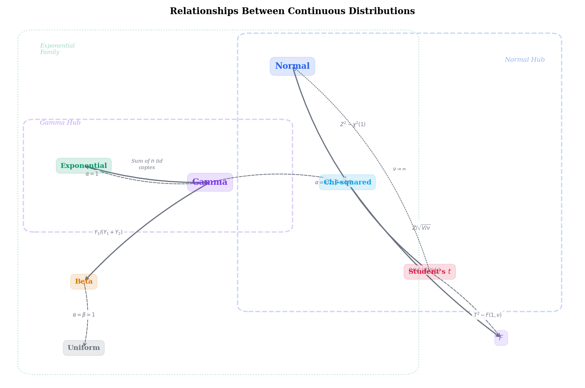
6.8 Relationships Between Distributions
The eight distributions form a rich web of connections. Rather than a single tangled graph, the relationships organize around two hubs.
Remark 8 Two-Hub Relationship Structure
The Gamma Hub. The Gamma distribution subsumes:
Exponential(λ)=Gamma(1,λ) — shape α=1
χ2(k)=Gamma(k/2,1/2) — shape α=k/2, rate β=1/2
Sum of iid Exponential(β): X1+⋯+Xn∼Gamma(n,β)
If Y1∼Gamma(α,1) and Y2∼Gamma(β,1) are independent, then Y1/(Y1+Y2)∼Beta(α,β)
The Normal Hub. The Normal distribution generates:
Z2∼χ2(1) — connects the Normal to the Gamma hub
Z/V/ν∼t(ν) — the Student’s t construction
(U/d1)/(V/d2)∼F(d1,d2) — the F construction from Chi-squareds
The two hubs are connected via the Chi-squared, which belongs to both (it is a Gamma special case and it is a sum of squared Normals).
Limit relationships:
t(ν)→N(0,1) as ν→∞
χ2(k)/k→1 as k→∞ (by the law of large numbers)
Gamma(α,β) with α→∞ and β=α/μ converges to N(μ,μ2/α)
6.9 Connections to ML
Example 6 KDE with Gaussian Kernel
Kernel Density Estimation places a small Normal bump Kh(x−xi)=h1φ(hx−xi) at each data point xi and averages:
f^(x)=n1i=1∑nh1φ(hx−xi)
The bandwidth h controls the bias-variance tradeoff: small h gives a spiky estimate (low bias, high variance), large h gives a smooth estimate (high bias, low variance). The Normal PDF’s smoothness and infinite support make it the default kernel. Kernel Density Estimation (Topic 30) develops the full theory, including the AMISE bias-variance decomposition, the AMISE-optimal bandwidth h∗=O(n−1/5), Epanechnikov’s optimal-kernel theorem, and data-driven bandwidth selectors (Silverman, Scott, UCV, Sheather-Jones). Topic 30 §30.6 is the featured section.
Example 7 The t-Test: Comparing Means with Unknown σ
Given n observations from N(μ,σ2) with σ2 unknown, we form:
T=S/nXˉ−μ0∼t(n−1)under H0:μ=μ0
where S is the sample standard deviation. The t distribution accounts for the uncertainty in estimating σ — its heavier tails (compared to the Normal) make the test less likely to reject when n is small. As n grows, t(n−1)≈N(0,1) and the distinction vanishes. Hypothesis Testing develops this rigorously, including the one- and two-sample t-tests; the two-sample F-test for equality of variances is covered in Linear Regression.
Example 8 Distribution Choice Guide
Choosing the right distribution for a modeling problem is a core ML skill:
Data type
Common choice
Why
Continuous, unbounded, symmetric
Normal
CLT, squared-error loss
Continuous, positive, right-skewed
Gamma or Log-Normal
Positive support, flexible skew
Waiting times, constant rate
Exponential
Memoryless property
Proportions, probabilities
Beta
Support on [0,1], conjugacy
Variance ratios, model comparison
F
Ratio of Chi-squareds
Small-sample means, unknown σ
Student’s t
Heavier tails than Normal
The key question is not “which distribution fits best?” but “which generative story matches my data?” The PDF shape is a consequence of the mechanism, not the other way around.
Summary
Eight continuous distributions, two structural hubs, one unifying theme: each distribution arises from a specific probabilistic mechanism, and the tools from Expectation, Variance & Moments — E[X], Var(X), MGF — reveal their properties.
Distribution
PDF kernel
E[X]
Var(X)
MGF
Exp. Family?
Uniform(a,b)
b−a1
2a+b
12(b−a)2
t(b−a)etb−eta
No
Normal(μ,σ2)
e−(x−μ)2/(2σ2)
μ
σ2
eμt+σ2t2/2
Yes
Exponential(λ)
λe−λx
λ1
λ21
λ−tλ
Yes
Gamma(α,β)
xα−1e−βx
βα
β2α
(β−tβ)α
Yes
Beta(α,β)
xα−1(1−x)β−1
α+βα
(α+β)2(α+β+1)αβ
—
Yes
χ2(k)
xk/2−1e−x/2
k
2k
(1−2t)−k/2
Yes
t(ν)
(1+t2/ν)−(ν+1)/2
0
ν−2ν
—
No
F(d1,d2)
—
d2−2d2
complex
—
No
What comes next. This topic cataloged the continuous distributions. The parallel treatment continues:
Exponential Families unifies the four exponential family members here with the five from Discrete Distributions, identifying natural parameters, sufficient statistics, and log-partition functions
Multivariate Distributions extends the Normal to the multivariate Normal — the star of that topic — and develops joint, marginal, and conditional densities in p dimensions
Bayesian Foundations (Topic 25) develops the Beta-Bernoulli, Gamma-Poisson, and Normal-Normal conjugate pairs in full generality, adds Normal-Normal-Inverse-Gamma (unknown σ²) and Dirichlet-Multinomial, and frames them all as instances of the exponential-family conjugacy theorem
Order Statistics & Quantiles shows that order statistics of Uniform(0,1) are Beta-distributed — §29.3 Theorem 2 + Corollary 1 give the full result via the probability-integral transform
Hypothesis Testing uses the Chi-squared, Student’s t, and F as test statistic distributions
![Gallery of all eight continuous distribution PDFs with E[X] balance-point triangles](/images/topics/continuous-distributions/continuous-distribution-catalog.png)