Sufficient Statistics & Rao-Blackwell
Data reduction, UMVUE, and the Pitman-Koopman-Darmois characterization — the theorems that close classical estimation.
16.1 From §7.6 to a Theory of Data Reduction
Topic 7 §7.6 stated the Fisher-Neyman factorization theorem only for exponential families: for a family of the form , the statistic is sufficient by construction — the factorization is already in the form the theorem demands. Topic 16 generalizes this to arbitrary dominated families and builds the full machinery of data reduction: minimal sufficiency, completeness, Rao-Blackwell optimality, the Lehmann-Scheffé UMVUE theorem, Basu’s independence theorem, and — closing the circle — the Pitman-Koopman-Darmois converse.
The thesis of the topic is one sentence: a sufficient statistic is exactly the data summary that loses nothing about the parameter, and exponential families are the only families where the summary stays small. Everything else — Rao-Blackwell, Lehmann-Scheffé, Basu — sharpens this into operational tools for building optimal estimators.
The concept of sufficiency originates with R. A. Fisher’s 1922 paper, On the Mathematical Foundations of Theoretical Statistics (§7 of that paper introduces “sufficient statistics” as one of the cornerstones of his program). Fisher’s argument was operational: estimators that ignore the sufficient statistic discard usable information, and one should prefer those that don’t. The measure-theoretic formalization — the modern statement and proof of the factorization theorem in full generality — came nearly thirty years later in Halmos & Savage (1949), Application of the Radon-Nikodym Theorem to the Theory of Sufficient Statistics. The Halmos–Savage paper handles the dominated-family case rigorously via the Radon–Nikodym derivative, which is what Topic 16 §16.3 quietly invokes when it speaks of densities for a common dominating measure .
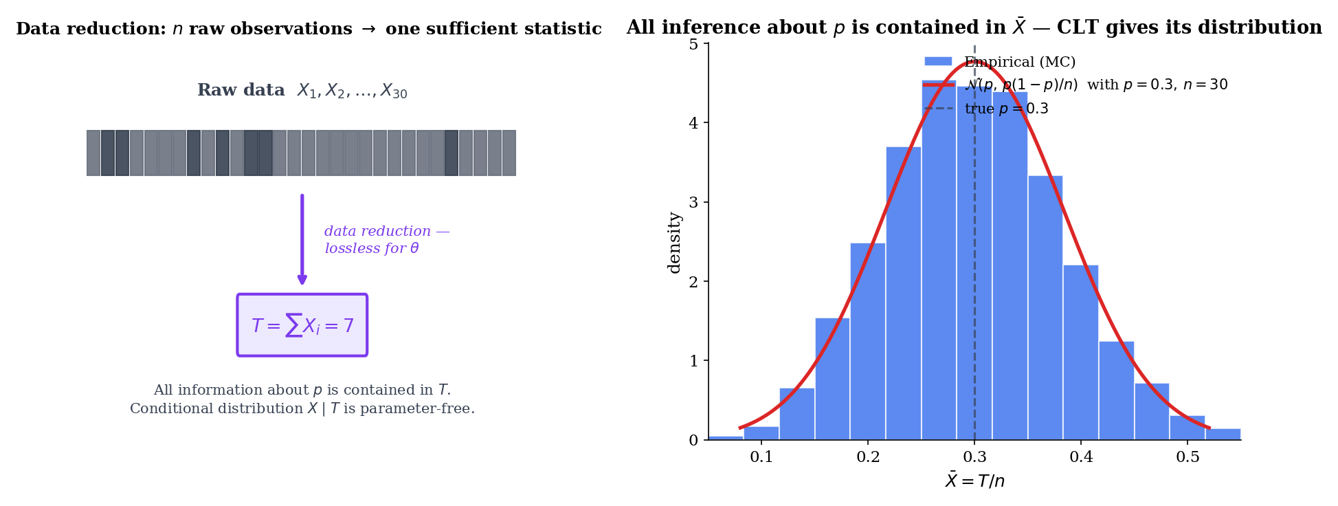
Sufficiency is a strong claim: is a lossless compression of the data with respect to . Once you know , the rest of the data is parameter-free noise — the conditional distribution does not depend on at all. This is information-theoretic in spirit but does not require Shannon information; it is a structural statement about the family . The compression is sometimes dramatic — for Bernoulli trials, the sufficient statistic is a single integer in ; for Normal observations with both parameters unknown, it’s a 2-vector . Topics 7, 13, 14, and 15 used this fact implicitly. §16.10 will reveal why the compression stays small only in exponential families.
16.2 Sufficient Statistics: The Conditional-Distribution Definition
The cleanest definition of sufficiency uses conditional distributions directly — no factorization theorem yet, no exponential-family scaffolding. The conditional distribution of the data given a sufficient statistic is parameter-free; everything else is downstream.
A statistic is sufficient for if the conditional distribution of given does not depend on — that is, is the same for every and every in the range of .
Operationally: knowing leaves no further parameter information in the data. The residual randomness of is “noise” in the strict sense that its distribution is fixed regardless of the truth.
A vector statistic is jointly sufficient for a parameter if the conditional distribution of given does not depend on . The dimension of the sufficient statistic need not equal the parameter dimension — though when is minimal (§16.4), and the family is regular (§16.10), the two dimensions match.
For iid data from any common distribution , the order statistic is sufficient for . Topic 29 makes the order statistic the central object of nonparametric statistics — Track 8 begins there precisely because this theorem tells us no nonparametric procedure ever discards information in the sorted sample.
The reason is structural: the iid joint density is symmetric in the arguments, so for every permutation . Conditioning on the order statistic is equivalent to conditioning on the unordered sample — and given the unordered sample, the distribution over labelings is uniform over all permutations regardless of . The order statistic is sufficient by construction. It is rarely minimal — for most families, a much smaller statistic also suffices.
Let be iid with known. Define . We check sufficiency directly: the conditional density of given is
The numerator is the iid Normal density . Expanding the squared-deviation sum,
The denominator is the density of , which contains the same term and the same term. The two cancel exactly, leaving the conditional density independent of . Hence is sufficient.
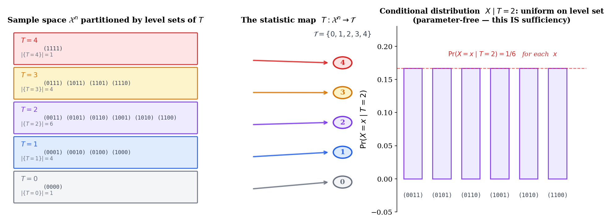
Let be iid , and define . The joint pmf is where . Conditional on , every binary vector with has probability
uniform over the vectors in the level set. The conditional is parameter-free — is sufficient.
The constant statistic is trivially sufficient: the “conditional distribution of given ” is just the marginal joint distribution of , which depends on in general — so this is not a counterexample, just a degenerate case of the definition. The genuinely degenerate sufficient statistic is the identity, itself, which is sufficient because conditioning on the full data leaves nothing to vary. Both extremes — too coarse to compress, too fine to compress — motivate minimal sufficiency (§16.4): the coarsest sufficient statistic that still captures everything.
The conditional-distribution definition (Def 1) is conceptually clean but operationally heavy — checking it requires writing out the joint density and dividing through, as in Examples 1 and 2. The Fisher–Neyman factorization theorem (§16.3) gives an equivalent and easier operational test: is sufficient iff the joint density factors as . The two definitions agree for dominated families (the standard setting), with the equivalence proved in §16.3. From here forward, factorization is the tool of choice; the conditional definition is the conceptual anchor.
16.3 The Fisher-Neyman Factorization Theorem
The factorization theorem is the engine of everything downstream. It converts the conditional-distribution definition (which requires checking that conditional densities are constant in ) into a one-line algebraic check on the joint density itself.
Let be a family of distributions on a measurable space , dominated by a common -finite measure , with densities . A statistic is sufficient for if and only if there exist non-negative measurable functions on and on such that
The factorization splits the joint density into a -dependent factor that touches the data only through and a -independent factor that absorbs everything else. The proof, which we give in full below, is direct in the discrete case and extends to the dominated case via Halmos–Savage.
Proof [show]
Discrete case (sufficiency factorization).
( Factorization sufficient.) Suppose . For any in the support and ,
The denominator is , since is constant on the level set. Substituting,
The conditional probability is a function of alone — no dependence — so is sufficient.
( Sufficient factorization.) Suppose is sufficient. Then does not depend on . Define
for any fixed reference . By sufficiency, does not depend on the choice of . Then
which is the desired factorization.
Continuous / dominated-family case. The discrete argument extends to the dominated-family setting via the Radon–Nikodym theorem. Let be a -finite measure dominating , so . The conditional density is well-defined as a Radon–Nikodym derivative on the level set , and sufficiency means this derivative does not depend on . The same algebra carries through with sums replaced by integrals: becomes the marginal density of , and becomes the conditional density of given — both well-defined on a -conull set.
∎ — using the conditional-probability definition (§2) and the dominated-family assumption (Halmos & Savage, 1949).
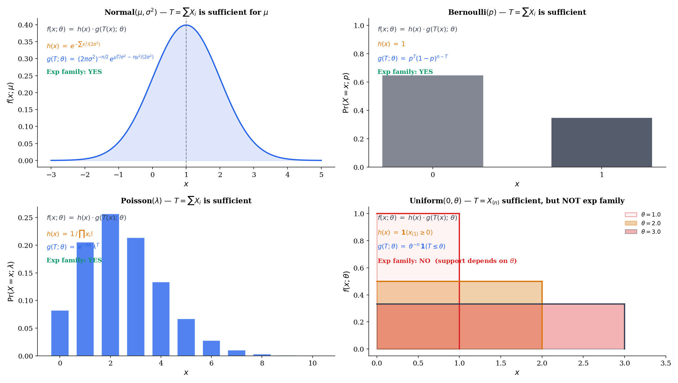
For iid with both parameters unknown, the joint density expands to
Setting and , the parameter-dependent factor is and the data-only factor is . Hence is jointly sufficient — a 2-vector matching the parameter dimension.
For iid , the joint density is
so is sufficient by factorization. The factorization is clean — but the family is not an exponential family: the support depends on , the support indicator cannot be absorbed into the exp-family form, and Topic 7’s construction does not apply. This example will return in §16.10 as the canonical counterexample to the Pitman–Koopman–Darmois theorem: a non-exp-family with a fixed-dimensional sufficient statistic, escaping the converse only by violating the regularity condition that support not depend on .
For iid , the joint pmf is
so is sufficient. As an exponential family in canonical form , the natural sufficient statistic is exactly this sum.
Compare Example 1 (the direct conditional check for Normal , which required expanding the squared-deviation sum and showing two terms cancel) with Example 4 (the factorization, which is two lines). For most families that arise in practice, factorization gives the sufficient statistic immediately by inspection: write down the joint density, group terms by -dependence, and read off . The conditional-distribution definition remains the conceptual anchor — it tells us why sufficiency means data reduction — but the factorization theorem is what we compute with.
16.4 Minimal Sufficiency
Sufficiency is closed under invertible (and even non-invertible) refinement: if is sufficient, so is , the order statistic, or any other statistic from which can be recovered. We want the coarsest sufficient statistic — the one that summarizes maximally without losing parameter information.
A sufficient statistic is minimal sufficient for if, for every other sufficient statistic , there exists a measurable function with almost surely. Equivalently, the partition of the sample space induced by is the coarsest partition under which sufficiency holds.
Suppose the family has densities with respect to a common dominating measure. A statistic is minimal sufficient for if and only if, for every pair of sample points ,
The forward direction is clear: if is minimal sufficient and , then and lie in the same level set of every sufficient statistic, so the likelihood ratio cannot distinguish -dependence at from . The converse — that any statistic with this likelihood-ratio constancy property is minimal sufficient — uses sufficiency of (the level sets give a sufficient partition, by factorization) plus the minimality of the partition (any coarser partition would merge points with -varying likelihood ratios, breaking sufficiency). The proof is short but technical; we omit the algebra here and refer to Casella & Berger (2002, §6.2.2).
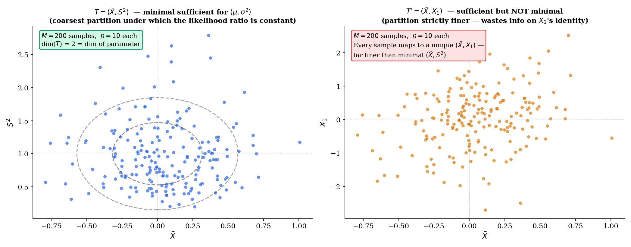
For iid Normal data with both parameters unknown, the likelihood ratio is
This is constant in if and only if AND — equivalently, AND . By Theorem 3, is minimal sufficient. The dimension matches the parameter dimension — a feature shared by every regular exponential family (and forced, under regularity, by Pitman–Koopman–Darmois).
For Normal data with known, is minimal sufficient. The expanded statistic is also sufficient (any function from which can be recovered inherits sufficiency), but it is not minimal: for any pair of samples with but , the likelihood ratio is constant in (since the joint density depends on only through ), but . Theorem 3’s biconditional fails, so is not minimal. Carrying along is information-wasting: it refines the partition without buying any inferential content.
A theorem due to Bahadur (1957) states that a complete sufficient statistic is minimal sufficient. The converse is false: the standard counterexample is Uniform, where the minimal sufficient statistic is not complete (Example 13, §16.6). Completeness is a strictly stronger property than minimality. The Lehmann–Scheffé theorem (§16.7) requires completeness, not just minimality, because it needs to rule out the existence of multiple unbiased functions of — and minimality alone does not.
16.5 The Rao-Blackwell Theorem
Sufficiency is structural — it identifies which summaries preserve parameter information. Rao–Blackwell makes it operational: any unbiased estimator can be improved (in the MSE sense) by conditioning on a sufficient statistic. The improvement is constructive and tight: it strictly reduces variance unless the estimator was already a function of .
Given an estimator and a sufficient statistic , the Rao-Blackwellized estimator is
By sufficiency, the conditional distribution of does not depend on , so the conditional expectation is a function of alone (not of ) — hence a statistic. The construction is constructive: integrate against the parameter-free conditional distribution .
Let be sufficient for and let be an unbiased estimator of with finite variance. Define . Then:
- is a statistic (function of alone).
- is unbiased: .
- , with equality iff almost surely (i.e., was already a function of ).
Since both estimators are unbiased, MSE = variance, so .
Proof [show]
Step 1 — is a statistic. The conditional distribution of given depends on only through (because is sufficient and is a function of ), and crucially does not depend on . So is computable without knowing — it is a function of alone.
Step 2 — is unbiased. By the law of iterated expectation (Topic 4),
Step 3 — via Eve’s law. The law of total variance (Eve’s law, Topic 4) decomposes the variance of as
Substituting ,
The first term is non-negative, with equality if and only if almost surely — i.e., is constant given , which means is itself a function of . Otherwise, strictly.
Since both estimators are unbiased, MSE equals variance, so — strictly so whenever was not already a function of .
∎ — using sufficiency of (Def 1), iterated expectation, and Eve’s law (Topic 4).
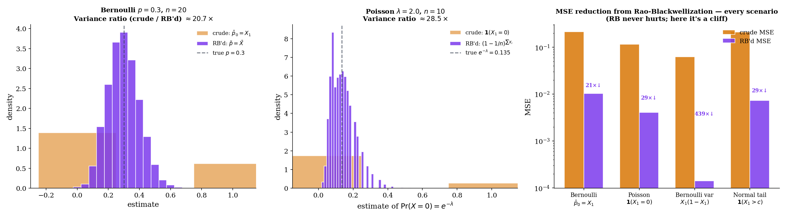
MSE(RB'd) = 0.0107
Ratio = 20.2×
For iid with sufficient, the crude estimator is unbiased () but lies in — variance is , the maximum possible for an estimator with this support. Conditioning on :
since by exchangeability all have the same conditional distribution given , and their conditional sum is . The Rao-Blackwellized estimator is the sample mean, with — a factor smaller than . The RaoBlackwellImprover above visualizes this dramatic shrinkage at .
Suppose we want to estimate from iid data. The crude estimator is unbiased (), but it is a 0/1 indicator. Conditioning on (which is ):
The conditional distribution of given is . So , and . The Rao-Blackwellized estimator is
which is the UMVUE of (since is complete sufficient — see §16.6 Lemma 1 — and Lehmann–Scheffé applies). A 0/1 estimator promoted to a smooth, sample-size-aware estimator with provably minimum variance among unbiased estimators.
Suppose we want to estimate for iid with known. The crude estimator is unbiased () but uses only one observation. Conditioning on the sufficient statistic :
by exchangeability of given . The variance ratio is — a factor- reduction. We finish this calculation in §16.7 Example 14, where Lehmann–Scheffé promotes it to the UMVUE.
Rao–Blackwell does more than prove the existence of a better estimator — it tells you exactly what it is: the conditional expectation , computable by integrating against the parameter-free conditional distribution . For the canonical families (Bernoulli, Poisson, Normal, Exponential, Gamma) the conditional distribution has a closed form, and the Rao-Blackwellized estimator is a direct calculation. This constructive aspect is what makes the theorem operational: Rao (1945) and Blackwell (1947) independently realized that every unbiased estimator can be mechanically upgraded by this recipe, without needing to know whether a UMVUE even exists.
16.6 Completeness
Rao–Blackwell guarantees that conditioning on a sufficient statistic does not hurt. But it does not guarantee uniqueness: two different unbiased estimators might Rao-Blackwellize to two different unbiased functions of . Completeness is the structural property that closes this gap — it says no two distinct unbiased functions of can have the same expectation, so the Rao-Blackwellization map is injective on unbiased functions.
A family of distributions of a statistic is complete if, for every measurable function with for all ,
A statistic is complete sufficient for if it is sufficient and the family of its distributions is complete. The statistic is boundedly complete if the implication above holds for every bounded measurable . Bounded completeness is strictly weaker than full completeness, and in fact suffices for the Lehmann–Scheffé theorem (§16.7 Remark 7).
Let be the canonical sufficient statistic of an exponential family with natural parameter ranging over an open subset . Then is complete for .
The argument is a one-liner: for every in the open set implies, by the uniqueness of the Laplace transform of the signed measure on , that almost everywhere under the dominating measure . The technical details (open natural parameter space, analyticity of , appropriate moment conditions) are handled rigorously in Brown (1986, §2.2). For our purposes, the operational consequence is clean: every full-rank exponential family with an open natural parameter space has a complete sufficient statistic, and Lehmann–Scheffé will deliver the UMVUE in every such family.
![Completeness demonstration. Left: Bernoulli (complete) — four candidate test functions g₁, g₂, g₃, g₄ of T = ΣXᵢ plotted as 𝔼_p[g(T)] vs p; only the constant-zero function gives the flat zero curve. Right: Uniform(θ, θ+1) (incomplete) — the range-based witness g(T) = (X_(n) − X_(1)) − (n−1)/(n+1) plotted as 𝔼_θ[g(T)] vs θ — the curve is identically zero for all θ (since the range is ancillary for the location parameter θ), with a non-witness contrast g'(T) = X_(1) − 1/(n+1) plotted as a linear-in-θ reference line.](/images/topics/sufficient-statistics/completeness-demo.png)
For complete families, only the constant-zero function g₀ ≡ 0 produces a flat zero curve in 𝔼_θ[g(T)] vs. θ. Any other test function traces a non-trivial θ-dependence.
By Lemma 1, every exponential family in its natural parameter has a complete sufficient statistic. Concretely:
- Bernoulli(): is complete for .
- Binomial() with known: itself is complete for .
- Poisson(): is complete for .
- Normal() with known: is complete for .
- Normal() jointly: is complete for .
- Gamma() with known: is complete for .
- Exponential(): is complete for .
Each delivers a UMVUE via Lehmann–Scheffé (§16.7).
Consider iid — a unit-width interval shifted by . The minimal sufficient statistic is the pair — two-dimensional for a one-dimensional parameter, an immediate structural warning sign.
Why incompleteness? Because is a pure location parameter, the range is ancillary for : its distribution depends only on , not on . (Specifically, has mean and a -shaped density, both free of .) Therefore the centered range
satisfies for every — yet is not identically zero. This is the definition of incompleteness: a non-trivial function of with zero expectation under every .
The CompletenessProbe above lets you visualize this directly: choose Uniform, evaluate the centered range across the -grid, and see the empirical curve. By contrast, on the same grid a non-witness like traces a non-zero linear function of — illustrating the difference between an ancillary-derived witness (which makes incompleteness visible) and a generic test function (which does not).
The Lehmann–Scheffé theorem (§16.7) is usually proved using full completeness. But a closer look at the proof shows that only bounded completeness is needed — the only test functions that arise are differences between unbiased estimators of the same quantity, and these are bounded whenever both have finite second moment. Bounded completeness is strictly weaker than full completeness, and a small number of important families (notably some non-regular location-scale families) are boundedly complete without being completely complete. For the canonical exponential families in this topic, the distinction does not matter — all are fully complete by Lemma 1.
16.7 The Lehmann-Scheffé Theorem
Sufficiency reduces the data without loss; completeness reduces unbiased functions of the data without redundancy. Lehmann–Scheffé combines them into a uniqueness-and-optimality statement: the unique unbiased function of a complete sufficient statistic is the uniformly minimum-variance unbiased estimator.
An estimator of a parameter (or parametric function) is the uniformly minimum-variance unbiased estimator (UMVUE) if:
- is unbiased: for every .
- For every other unbiased estimator of , for every .
The “uniformly” applies to the parameter — the variance dominance must hold simultaneously at every , not just on average or at a particular value. UMVUE existence is non-trivial: there are families with no UMVUE at all (Remark 8). When a UMVUE exists, it is essentially unique (Theorem 6).
Let be a complete sufficient statistic for , and let be an unbiased estimator of that is a function of . Then is the unique UMVUE of .
Proof [show]
Existence (any unbiased estimator can be improved to a function of ). Let be any unbiased estimator of . Define . By the Rao–Blackwell theorem (Theorem 4), is a function of , is unbiased for , and has variance .
Uniqueness (any two unbiased functions of agree almost surely). Suppose and are both unbiased for . Then for every ,
By completeness of (Definition 5), this forces almost surely under every — that is, a.s.
Optimality (Rao-Blackwellization always lands on ). For any unbiased , the Rao-Blackwellization is an unbiased function of . By uniqueness, almost surely. Therefore
with the second inequality from Rao-Blackwell. This holds for every unbiased , so is the UMVUE — uniformly across and uniquely up to a.s. equality.
∎ — by Rao-Blackwell (Theorem 4) and completeness (Definition 5).
If a UMVUE of exists, then it is unique up to almost-sure equality under every — that is, any two UMVUE candidates and agree on a set of -measure 1 for every .
This is a corollary of Theorem 5: any UMVUE must be a function of any complete sufficient (otherwise Rao-Blackwellization strictly improves it), and any two unbiased functions of agree a.s. by completeness. Without completeness, the uniqueness conclusion fails — a family with multiple inequivalent UMVUEs exists in principle, but is exotic.
![Lehmann-Scheffé construction. Left: the Lehmann-Scheffé "diamond" — θ̂* (any unbiased) → θ̃ = 𝔼[θ̂* | T] (Rao-Blackwellized, function of T) → unique UMVUE (by completeness). Right: for Normal σ² known μ, histograms of crude σ̂² = (X₁ − μ)², RB'd σ̃² = Σ(Xᵢ − μ)²/n, with the variance-ratio = n annotation.](/images/topics/sufficient-statistics/lehmann-scheffe-construction.png)
Let be iid with known and unknown. The complete sufficient statistic is , which has distribution . The unbiased function of for is
since . By Lehmann–Scheffé (Theorem 5), this is the UMVUE of in this model. Variance: — exactly the CRLB (Topic 13 §13.7). The UMVUE is efficient in this case.
Note the crucial assumption known. With unknown the model is exactly the same family but with two parameters, and the complete sufficient statistic becomes — leading to the famous Bessel correction; see Example 19 below.
Let be iid with shape known and rate unknown — an exponential family in . The complete sufficient statistic is , with for (a standard Gamma reciprocal-moment identity). Hence the unbiased function of for is
By Lehmann–Scheffé this is the UMVUE. Compare with the MLE / MoM: . The two estimators differ by exactly the bias-correction factor — a small but non-trivial gap that the §16.11 UMVUEComparator visualizes. This is the example that fulfills the method-of-moments.mdx:1062 promise.
Two cautions worth flagging. First, a UMVUE need not exist. In families without a complete sufficient statistic, the set of unbiased estimators may have no member that uniformly dominates the others — the Lehmann–Scheffé existence proof relies critically on completeness. Second, even when the UMVUE exists, it does not always attain the Cramér–Rao lower bound. The CRLB is a bound on variance, derived from the information inequality; UMVUE is the best unbiased estimator. The UMVUE attains the CRLB precisely in full-rank exponential families with the parameter being the natural one — exactly the same condition for which MLE = UMVUE = MoM coincide (§16.11 Theorem 9). Outside that boundary, the UMVUE has variance strictly above the CRLB, and the gap measures the unattainability of efficient estimation in that family.
16.8 UMVUE Worked Examples
The Lehmann–Scheffé theorem turns sufficiency + completeness into an algorithm: identify the complete sufficient statistic, find an unbiased function of it, and you have the UMVUE. The five canonical examples below demonstrate the algorithm and lay the ground for §16.11’s triple-estimator comparison.
| Family | Parameter | UMVUE | MLE | MoM | Relationship |
|---|---|---|---|---|---|
| Bernoulli() | triple coincidence | ||||
| Poisson() | triple coincidence | ||||
| Normal() | ( known) | triple coincidence | |||
| Normal() | ( unknown) | UMVUE MLE = MoM | |||
| Exponential() | UMVUE MLE = MoM | ||||
| Gamma(), known | UMVUE MLE = MoM |
is complete sufficient for , and , so . The MLE is also (Topic 14, Example 14.1), and so is the MoM (Topic 15, Example 15.3). All three coincide — the Bernoulli is exp family in its natural parameter, so Theorem 9 (§16.11) applies. Variance: , which equals the CRLB — efficient.
is complete sufficient for , and , so . The MLE (Topic 14, Example 14.4) and MoM (Topic 15, §15.2) both also equal . Triple coincidence again, and again CRLB-attaining: .
With known, is complete sufficient and unbiased for , hence the UMVUE. The MLE is also (Topic 14, Example 14.2 with fixed), and the MoM is too (Topic 15, Example 15.1). All three coincide; the variance equals the CRLB.
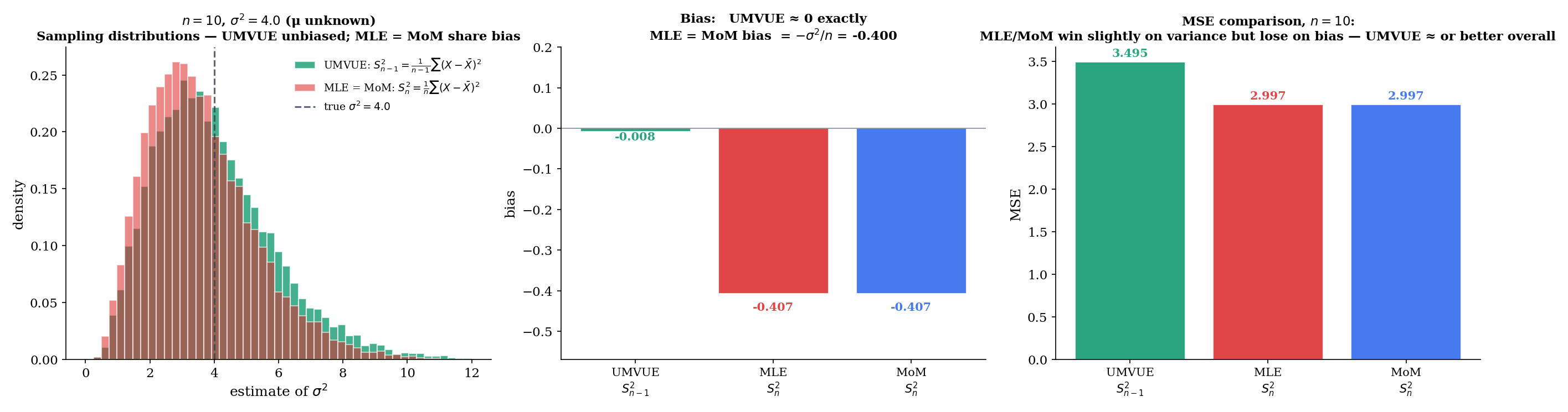
With also unknown, the complete sufficient statistic is the pair . The unbiased function of for is the Bessel-corrected sample variance,
since and . The MLE and MoM, by contrast, both land at the un-corrected
with bias . The bias is small but does not disappear: at and , the MLE/MoM bias is . The featured §16.11 comparison runs all three estimators in parallel and shows the UMVUE on top by a small but persistent margin in MSE for moderate .
Suppose we want to estimate for some fixed threshold . The crude unbiased estimator is the indicator . Conditioning on the complete sufficient , the UMVUE turns out to be a regularized incomplete-beta tail:
with the regularized incomplete beta function. This is the formula used by umvueNormalTailProb in estimation.ts. The full derivation (in Lehmann & Casella, 1998, §2.4) integrates the indicator against the conditional distribution of given , which has a scaled-Beta form. The point: even for non-trivial parametric functions, Rao-Blackwellization combined with completeness gives the UMVUE in closed form when the sufficient statistic has tractable conditional distributions.
Reading the table at the top of §16.8: in every exp-family in its natural parameter, UMVUE = MLE = MoM = (or its relevant linear transform). Outside the natural parameterization, UMVUE and MLE diverge in a structured way: UMVUE prioritizes unbiasedness ( for Normal ); MLE and MoM coincidentally prioritize a different summary (, the maximum-likelihood projection onto the tangent space) and pay a small bias cost. For finite , the comparison is family-specific: sometimes UMVUE wins on MSE (Normal at moderate ), sometimes MLE wins (e.g., Gamma scale in some regimes — its slight positive bias and lower variance can yield smaller MSE for very small ). Asymptotically, all three are consistent and asymptotically Normal at the same rate; the bias gap shrinks as , so it disappears in the asymptotic limit.
16.9 Ancillary Statistics and Basu’s Theorem
Sufficient statistics carry all the parameter information; ancillary statistics carry none of it. Basu’s theorem says that when the first is complete sufficient, the two are independent — a startlingly clean structural result with broad consequences in Track 5.
A statistic is ancillary for if its distribution under does not depend on — that is, is the same function of for every .
A statistic is first-order ancillary for if its mean does not depend on , even if higher moments might. First-order ancillarity is strictly weaker than full ancillarity. For most of our purposes — and for Basu’s theorem — we use full ancillarity.
Examples of ancillary statistics: the sample range for a pure-location family; the studentized statistic in a Normal family with location parameter and known shape; any function of standardized residuals after removing a location and scale.
If is a complete sufficient statistic for and is an ancillary statistic for , then and are independent under every .
Proof [show]
Fix any measurable event in the -algebra generated by . Define
The conditional probability does not depend on . Because is sufficient, the conditional distribution of (and hence of any function of , including ) given does not depend on . So is the same function of for every — it is a statistic.
The marginal probability does not depend on . Because is ancillary for , its distribution under does not depend on . So is a constant in .
Hence is a well-defined statistic (a function of minus a constant). Taking expectation under :
where the first equality uses iterated expectation. This holds for every . By completeness of , the implication a.s. forces
This is the definition of independence of and under , for every measurable — hence under , for every .
∎ — by sufficiency of , ancillarity of , and completeness (Definition 5).
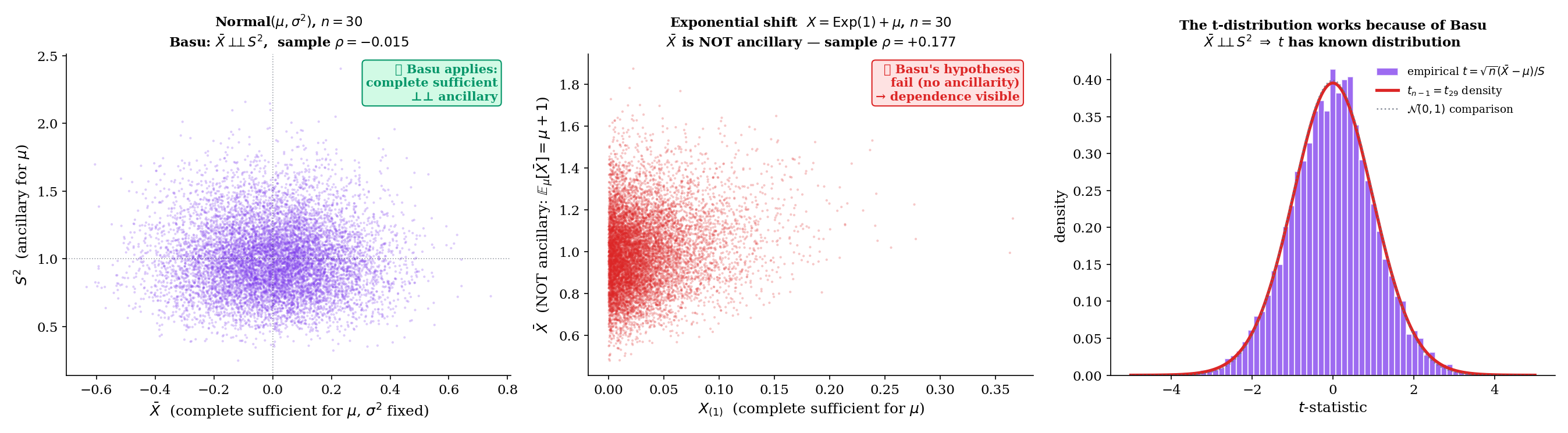
Theoretical: 0 (Basu)
If T is complete sufficient for θ and A is ancillary for θ, then T ⊥⊥ A under every P_θ. Visualized as: their joint MC scatter should be decorrelated — sample ρ ≈ 0.
For iid with fixed and known, is complete sufficient for . The sample variance has distribution , which depends on but not on — so is ancillary for at fixed . By Basu’s theorem,
This is the independence that makes the t-statistic have a well-defined distribution: it’s the ratio of an independent (from ) and (from ) — exactly the construction of Student’s . The t-test, the t-confidence-interval, and the entire Track 5 chapter on hypothesis testing for Normal-mean problems all rest on this Basu corollary. The BasuIndependence component above visualizes this independence as a decorrelated MC scatter cloud.
For iid , is complete sufficient for (a standard exercise — completeness follows from the fact that any zero-expectation function must satisfy for all , which by differentiation in forces on ). The ratio has distribution regardless of — pure scale-equivariance — so is ancillary. Basu’s theorem then gives , a non-obvious consequence of the structure of order statistics. (The uniform-order-statistics structure this exploits is developed in Topic 29 §29.3.) This kind of independence underlies many likelihood-ratio test statistics and pivotal quantities for scale parameters.
The independence in Example 21 is the technical engine of one-sample Normal inference. Without it, the ratio would have a distribution depending on the joint distribution of in a complicated way; with it, the ratio becomes the textbook . Track 5 (hypothesis testing) and Track 5.5 (confidence intervals) build the t-test, the F-test, and the analysis of variance on this foundation. Basu provides the abstract reason: complete sufficiency for one parameter (, with fixed) plus ancillarity for that parameter (, whose distribution doesn’t depend on ) gives independence, which is exactly what pivotal-quantity inference needs. We will return to this when we develop the t-test in Track 5.
16.10 The Pitman-Koopman-Darmois Theorem
The classical results so far — sufficiency, completeness, Rao-Blackwell, Lehmann-Scheffé, Basu — work for any family that has a complete sufficient statistic. The Pitman–Koopman–Darmois theorem is the converse direction: it says that, under regularity, the only families admitting fixed-dimensional sufficient statistics for iid samples of every size are the exponential families.
In other words: Topic 7’s exponential families are not just one class with nice data-reduction properties — they are the only class. This converts Topic 7’s “exponential families are convenient” into “exponential families are essentially forced” — a structural result with serious philosophical weight.
Let be a family of densities on with respect to Lebesgue measure, and assume:
- (A) The support is independent of .
- (B) on .
- (C) is twice continuously differentiable in jointly on .
Suppose, in addition, that for every sample size , there exists a scalar-valued sufficient statistic for (i.e., a real-valued function, not a vector). Then is an exponential family in canonical form:
for some twice continuously differentiable functions , , , and .
Proof [show]
Step 1 — Apply Fisher–Neyman to the iid joint density. By Theorem 2 (Fisher–Neyman factorization), sufficiency of means
Taking logs:
Step 2 — Differentiate in . Differentiating both sides with respect to (which is allowed because of (B) and (C)),
The left-hand side is a sum of one-variable functions . The right-hand side depends on only through the scalar . This functional-form constraint will force the structure.
Step 3 — Cross-differentiate in . Fix any and differentiate both sides with respect to :
The left-hand side depends only on the pair ; the right-hand side depends on only through and the partial . For this equation to hold for every choice of and every , the structural form must separate: there exist differentiable functions and such that
(This step is the content of the original Darmois (1935) argument; the careful version handles the case on a measure-zero set.)
Step 4 — Integrate in . Integrating the previous equation in ,
where is the “constant of integration in ” — a function of alone.
Step 5 — Integrate in . Integrating in ,
where is the “constant of integration in .” Exponentiating:
where and . This is the canonical exponential-family form (Topic 7 §7.3) with natural parameter , sufficient statistic , log-partition , and base measure .
∎ — via Fisher–Neyman (Theorem 2) and the separable functional equation derived in Steps 3–5.
![PKD theorem schematic. Left: schematic of the PKD theorem's logic — "regular family with fixed-dim sufficient statistic for every n" ⟹ "exponential family"; inverse arrow "Topic 7: exp families HAVE fixed-dim sufficient statistics". Right: the Uniform(0, θ) counterexample — support [0, θ] shown with θ-dependent right endpoint (shaded region changes with θ), annotation "support depends on θ — violates PKD regularity (A); Uniform is NOT an exponential family despite having 1-dim sufficient statistic X_(n)".](/images/topics/sufficient-statistics/pkd-theorem.png)
Consider iid . By Example 5, is sufficient (scalar, fixed-dimensional, for every ). Yet this family is not an exponential family — and the PKD theorem’s regularity (A) tells us why: the support depends on , so (A) fails. The cross-differentiation step in the proof relies on on a -independent set, and this fails at the boundary . Without (A), the PKD conclusion does not apply, and Uniform escapes the conclusion despite having a fixed-dim sufficient statistic.
The lesson: the regularity conditions in PKD are not technical decorations — they are the price of the structural conclusion. Drop the support condition and the converse fails. The non-exp families with fixed-dim sufficient statistics that arise in practice (Uniform endpoints, truncated families, exponential shifts) are exactly those whose support varies with the parameter.
The scalar Theorem 8 generalizes to with a -dimensional sufficient statistic. The regularity (A)–(C) conditions extend in the obvious way (support independent of , twice differentiability), and the new condition is a Jacobian-rank requirement: the matrix must have full rank on . Under these conditions, the family is a -parameter exponential family. The proof — which requires careful measure-theoretic regularity to handle the multi-dimensional integration — is the content of Brown (1986, §2.3). For our purposes, the scalar version is enough; the multiparameter generalization is a Remark, not a Theorem, in this topic.
Topic 7 introduced exponential families as a “convenient class with closed-form sufficient statistics, MLEs, and conjugate priors.” PKD reverses the direction: under regularity, exponential families are the only such class. This is what makes the exp-family chapter foundational rather than ornamental — every regular family with bounded-dimensional sufficient statistics is, structurally, an exponential family. The catalog in Topic 7 (Bernoulli, Binomial, Poisson, Normal, Gamma, Beta, Multinomial, Dirichlet, etc.) is not a curated list of nice examples but an enumeration of all the families satisfying PKD’s regularity. This is why exponential families appear everywhere in machine learning — variational inference, generalized linear models, conjugate Bayesian computation, energy-based models — they are the structural attractor for “tractable + parametric + regular.”
16.11 UMVUE vs MLE vs MoM: The Estimator Landscape Closes
Track 4 began with the evaluation framework (Topic 13: bias, variance, MSE, consistency, asymptotic normality, efficiency, CRLB) and applied it to two estimation methods: maximum likelihood (Topic 14) and method of moments (Topic 15). Topic 16 has now added the third — UMVUE via Lehmann–Scheffé. §16.11 brings all three into a single comparison: where they agree, where they diverge, and what their differences tell us about bias, efficiency, and the geometry of the likelihood.
Let be a one-parameter exponential family with the natural parameter and the canonical sufficient statistic. Suppose is complete sufficient (Lemma 1) and the MoM equation selects the natural parameter directly (i.e., the MoM estimating equation is , the moment-matching identity from Topic 7 §7.8). Then
In particular, all three estimators coincide for Bernoulli(), Poisson(), Normal(, known) at the parameter , and any other exp-family in its natural parameterization with a one-to-one -map.
The proof is short: Topic 7 §7.8 showed solves the moment-matching identity , which is exactly the MoM equation solves. Lehmann–Scheffé (§16.7) gives that the unbiased function of for — when one exists — is the unique UMVUE. In the natural parameter case, is unbiased for , and the inversion is monotone, so the UMVUE coincides with the MLE.
This Theorem fulfills the method-of-moments.mdx:1062 promise: in exponential families in the natural parameter, the three estimation principles agree exactly. The interesting cases — and the focus of the UMVUEComparator below — are the families just outside this regime: Normal with unknown (where the MoM and MLE land on a different summary than the UMVUE), and Gamma scale with known shape (where the UMVUE applies a correction the MLE does not).
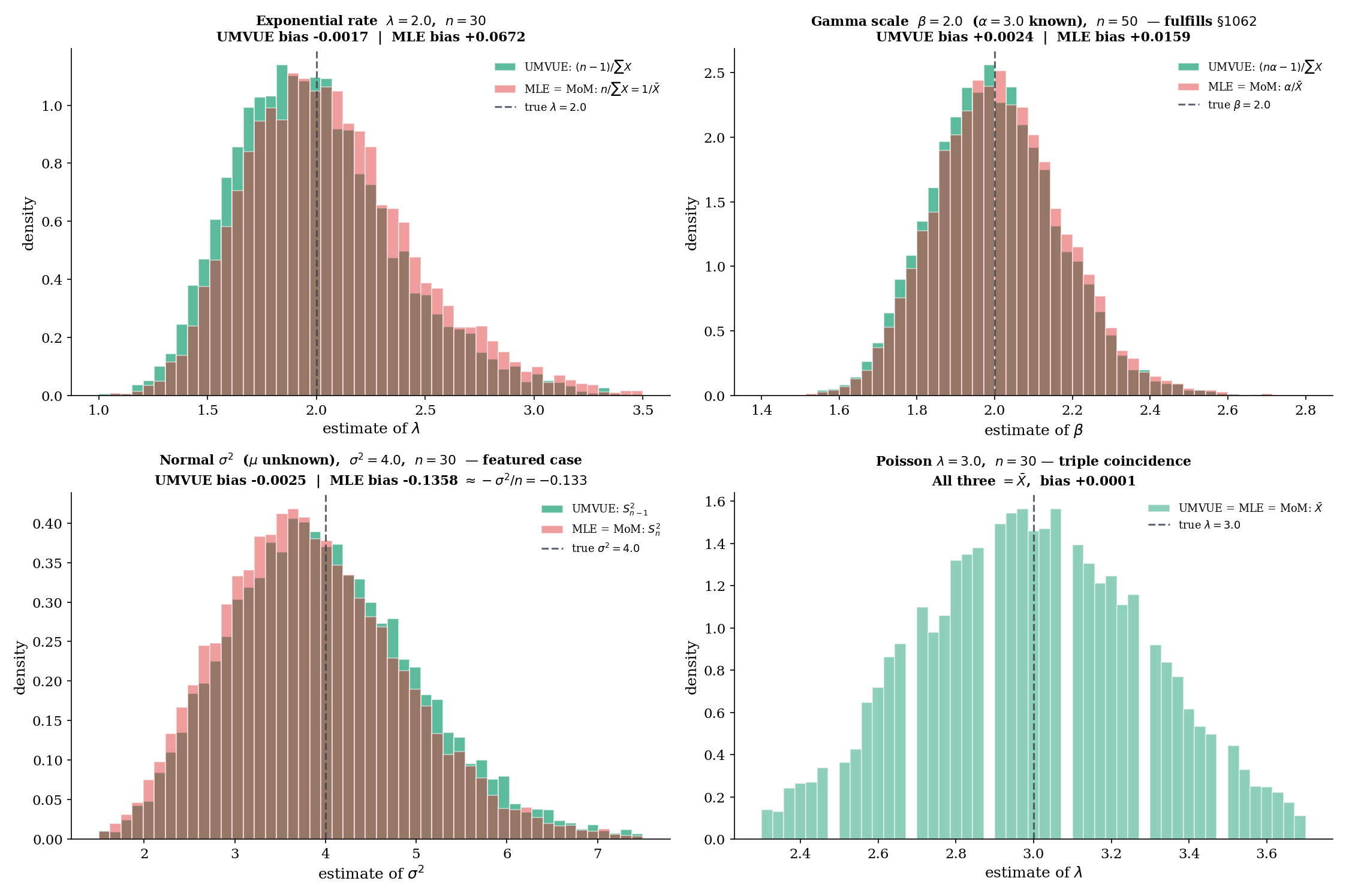
For iid , is complete sufficient and , with for . So the UMVUE is
The MLE and MoM both equal (Topic 14 Example 14.7; Topic 15 Example 15.2). The two differ by exactly the factor — a small but persistent bias gap. The UMVUE is strictly unbiased; the MLE/MoM has a small positive bias going to zero as . UMVUEComparator’s Exponential preset visualizes this: the three sampling distributions overlap heavily, but UMVUE sits exactly on while MLE/MoM are slightly displaced.
This is the example that fulfills the method-of-moments.mdx:1062 promise. For iid with known, the family is one-parameter exponential in (rate). is complete sufficient. The UMVUE is
while the MLE and MoM both equal . The bias-correction factor is exactly — a clean instance of the structural pattern: when the parameter is not the natural one (here rather than as the natural parameter), MLE/MoM and UMVUE differ in finite samples but agree asymptotically. The UMVUEComparator’s Gamma preset at , , shows the gap clearly: UMVUE bias , MLE/MoM bias , MSE close but UMVUE marginally better.
Returning to Example 19 with the full triple-comparison lens. UMVUE is (the Bessel-corrected variance, unbiased); MLE = MoM is (with bias ). At and , the bias gap is , the variance ratio is , and MSE comparison is dictated by
For and : MSE(UMVUE) , MSE(MLE/MoM) — slightly lower for the biased estimator. This is the small-sample regime where the bias-variance trade-off can favor the biased MLE; for larger , both MSEs collapse and the UMVUE’s strict unbiasedness wins. The UMVUEComparator’s Normal preset visualizes both regimes by varying .
Track 4 began with the evaluation framework (Topic 13) and asked: which estimators win on bias, variance, and MSE, and how do we know? Topics 14–16 answered this for the three classical methods.
- MLE (Topic 14): asymptotically efficient under regularity; consistency and asymptotic normality from the LLN/CLT machinery.
- MoM (Topic 15): simpler, sometimes equivalent to MLE (in exp families, exactly), often less efficient (ARE outside).
- UMVUE (Topic 16): the unique unbiased estimator with minimum variance, when complete sufficiency is available.
The three principles agree in exp families in their natural parameter (Theorem 9). They diverge in structurally interpretable ways outside: UMVUE prioritizes strict unbiasedness; MLE prioritizes asymptotic efficiency (with bias going to zero); MoM trades both for closed-form simplicity. The Normal unknown case is the canonical “all three differ” example, and §16.11 provides the synthesis.
Track 4 is now closed. Track 5 picks up the inferential toolkit — hypothesis testing, confidence intervals, Bayesian inference — built on top of the estimators we now have.
16.12 Where Sufficiency Falls Short
Sufficiency is foundational but not the whole story of inference. Three short remarks flag where its reach ends.
After sufficient-statistic-based reduction, an ancillary statistic can still provide a “more relevant reference set” for inference. Fisher’s conditionality principle says that inference for should be conducted conditional on the observed value of any ancillary statistic — even though the marginal distribution of the ancillary is parameter-free. This creates a tension: sufficiency reduces the data to for the model; ancillarity refines the inference to a relevant subset for interpretation. In a one-sample Normal location problem with known variance, the ancillary is trivial and the conditionality principle adds nothing. In more complex problems (e.g. linear regression with covariates that are themselves random), the ancillary is the design matrix and conditional inference becomes the standard frequentist approach. We take this up in Track 5 (confidence intervals via pivotal quantities) and again in the Bayesian track (the likelihood principle, where conditioning on ancillary statistics is equivalent to using the likelihood for inference).
The Lehmann–Scheffé machinery requires completeness, which in turn typically requires regularity (PKD assumption (A): support independent of ). Non-regular families — Uniform being the canonical example — escape PKD by violating (A), and Lehmann–Scheffé does not directly apply. Yet these families have minimum-variance unbiased estimators (MVUEs), constructed by different means. For Uniform, the MVUE is — a bias-correction of the MLE . The general theory of estimators in non-regular families is the Pitman estimator framework (named for the same Pitman as in PKD), which builds optimal equivariant estimators using the group structure of the parameter (location, scale, location-scale). Track 6 (linear regression and beyond) returns to this when discussing equivariant procedures for shifts and scales.
For non-exp families (no fixed-dim sufficient statistic), data reduction in the strict sense fails — the minimal sufficient statistic grows with . But asymptotic sufficiency rescues a weaker version: as , the MLE becomes asymptotically sufficient in the sense that all relevant inferential information concentrates on a finite-dimensional sufficient statistic tangent to the true parameter. This is the content of Le Cam’s Local Asymptotic Normality program: under regularity, the log-likelihood ratio sequence behaves locally like a Normal location family, and the MLE is the asymptotically efficient estimator. The framework unifies MLE asymptotic efficiency, Bayesian contraction rates, and the CLT into a single picture — and it generalizes to non-iid, non-parametric, and high-dimensional settings. Le Cam’s book (1986) and van der Vaart’s Asymptotic Statistics (1998) are the canonical references. The information-bottleneck and representation-learning topics on formalml.com pick up the same thread for learned (rather than computed) sufficient statistics.
16.13 Summary & Forward Look
| Concept | Definition | Inferential role |
|---|---|---|
| Sufficient | parameter-free | preserves all parameter info |
| Minimal sufficient | coarsest sufficient | no data redundancy |
| Complete | a.s. | no functional redundancy in |
| Ancillary | distribution free of | carries no parameter info |
| UMVUE | unbiased, min variance uniformly | Lehmann–Scheffé construction |
The lattice of implications: complete sufficient minimal sufficient (Bahadur 1957). Complete sufficient ancillary (Basu, Theorem 7). Lehmann–Scheffé combines completeness + sufficiency unique UMVUE (Theorem 5). Pitman–Koopman–Darmois closes the loop: under regularity, exp families are the only families with fixed-dim sufficient statistics for every (Theorem 8). Topic 7’s exp-family construction supplies the sufficient statistic; Topic 16 supplies the entire optimality theory built on top.
Closing Track 4. The classical estimation toolkit is now complete:
- Topic 13: the evaluation framework — bias, MSE, consistency, asymptotic normality, efficiency, Fisher information, CRLB.
- Topic 14: the maximum likelihood estimator — score equation, asymptotic efficiency, Newton-Raphson and Fisher scoring.
- Topic 15: the method of moments and M-estimation — closed-form moment matching, ARE comparison with MLE, the sandwich variance.
- Topic 16: sufficiency, completeness, Rao–Blackwell, Lehmann–Scheffé, Basu, and Pitman–Koopman–Darmois — the structural theory of optimal unbiased estimation, the converse to Topic 7’s exp families.
The three operative principles (UMVUE, MLE, MoM) coincide in exp families in the natural parameter (§16.11 Theorem 9) and diverge in structurally informative ways outside. Track 4 is closed.
Topic 16’s machinery is foundational for almost every downstream topic on this site and on formalml.com.
- Hypothesis Testing (Topic 17) — score tests, Wald tests, and likelihood-ratio tests are all functions of the sufficient statistic. The one-sample t-test derivation (§17.7 Thm 5) uses Basu’s independence directly, fulfilling the forward promise in Example 21 of this section. The Neyman–Pearson lemma is stated in Topic 17 §17.9 and proved in Topic 18.
- Confidence Intervals — pivotal quantities are constructed from ancillary statistics (Basu’s theorem gives the required independence); Wilks-type intervals use asymptotic sufficiency of the MLE.
- Bayesian Foundations (Topic 25) — the posterior depends on the data only through the sufficient statistic. Conjugate priors (Topic 7 §7.7) become especially natural when is complete sufficient — the posterior collapses to a finite-dimensional family.
- Linear Regression (Track 6) — OLS estimators are functions of — sufficient statistics for the Normal linear model. Gauss–Markov gives UMVUE among linear unbiased estimators; under Normal errors, this is the UMVUE.
- Generalized Linear Models — GLMs leverage exp-family sufficient statistics directly; iteratively reweighted least squares is a score-based algorithm that descends along the sufficient statistic’s geometry.
- formalml.com — Information bottleneck — the IB method finds a representation of that preserves information about a target . In the special case where , the IB recovers exactly the Topic 16 notion of sufficiency. Learned sufficient statistics are the deep-learning analog of the parametric ones we’ve built here.
- formalml.com — Representation learning — self-supervised contrastive and masked-modeling objectives implicitly discover sufficient statistics of for downstream tasks. The Rao–Blackwellization intuition (optimal estimators are functions of ) reappears as the rationale for pretrained-feature reuse.
The thread connecting all of these: sufficient statistics are the abstract object that data reduction discovers; everything else is downstream.
References
- Erich L. Lehmann & George Casella. (1998). Theory of Point Estimation (2nd ed.). Springer.
- George Casella & Roger L. Berger. (2002). Statistical Inference (2nd ed.). Duxbury.
- Lawrence D. Brown. (1986). Fundamentals of Statistical Exponential Families. IMS Lecture Notes Monograph Series, Vol. 9.
- Ronald A. Fisher. (1922). On the Mathematical Foundations of Theoretical Statistics. Philosophical Transactions of the Royal Society A, 222, 309–368.
- Paul R. Halmos & Leonard J. Savage. (1949). Application of the Radon-Nikodym Theorem to the Theory of Sufficient Statistics. Annals of Mathematical Statistics, 20(2), 225–241.
- C. Radhakrishna Rao. (1945). Information and the Accuracy Attainable in the Estimation of Statistical Parameters. Bulletin of the Calcutta Mathematical Society, 37, 81–91.
- David Blackwell. (1947). Conditional Expectation and Unbiased Sequential Estimation. Annals of Mathematical Statistics, 18(1), 105–110.
- Erich L. Lehmann & Henry Scheffé. (1950). Completeness, Similar Regions, and Unbiased Estimation — Part I. Sankhyā, 10(4), 305–340.
- Debabrata Basu. (1955). On Statistics Independent of a Complete Sufficient Statistic. Sankhyā, 15(4), 377–380.
- Georges Darmois. (1935). Sur les lois de probabilité à estimation exhaustive. Comptes rendus de l’Académie des Sciences, 200, 1265–1266.
- Bernard O. Koopman. (1936). On Distributions Admitting a Sufficient Statistic. Transactions of the American Mathematical Society, 39(3), 399–409.
- E. J. G. Pitman. (1936). Sufficient Statistics and Intrinsic Accuracy. Mathematical Proceedings of the Cambridge Philosophical Society, 32(4), 567–579.