Model Selection & Information Criteria
When every candidate model fits the training data differently, a principled ranking criterion is the only honest arbiter. AIC (Akaike) estimates out-of-sample log-likelihood asymptotically; BIC (Schwarz) approximates the Bayesian marginal likelihood; Mallows' Cp is the Gaussian special case; Stone's 1977 theorem identifies LOO-CV with AIC; Yang 2005 proves that selection consistency and prediction efficiency are mutually incompatible. Track 6 closes here.
24.1 The model-selection problem
Given data and a candidate family of statistical models — each with parameter space and likelihood — the model-selection problem is to choose one model from the family by a procedure that has a defensible asymptotic justification. Maximum log-likelihood alone is not such a procedure: is monotone in model complexity, so it always picks the largest candidate.
For an estimator trained on and a fresh observation from the same data-generating distribution, the prediction risk under loss is
For log-likelihood loss , the risk is the negative expected log-predictive
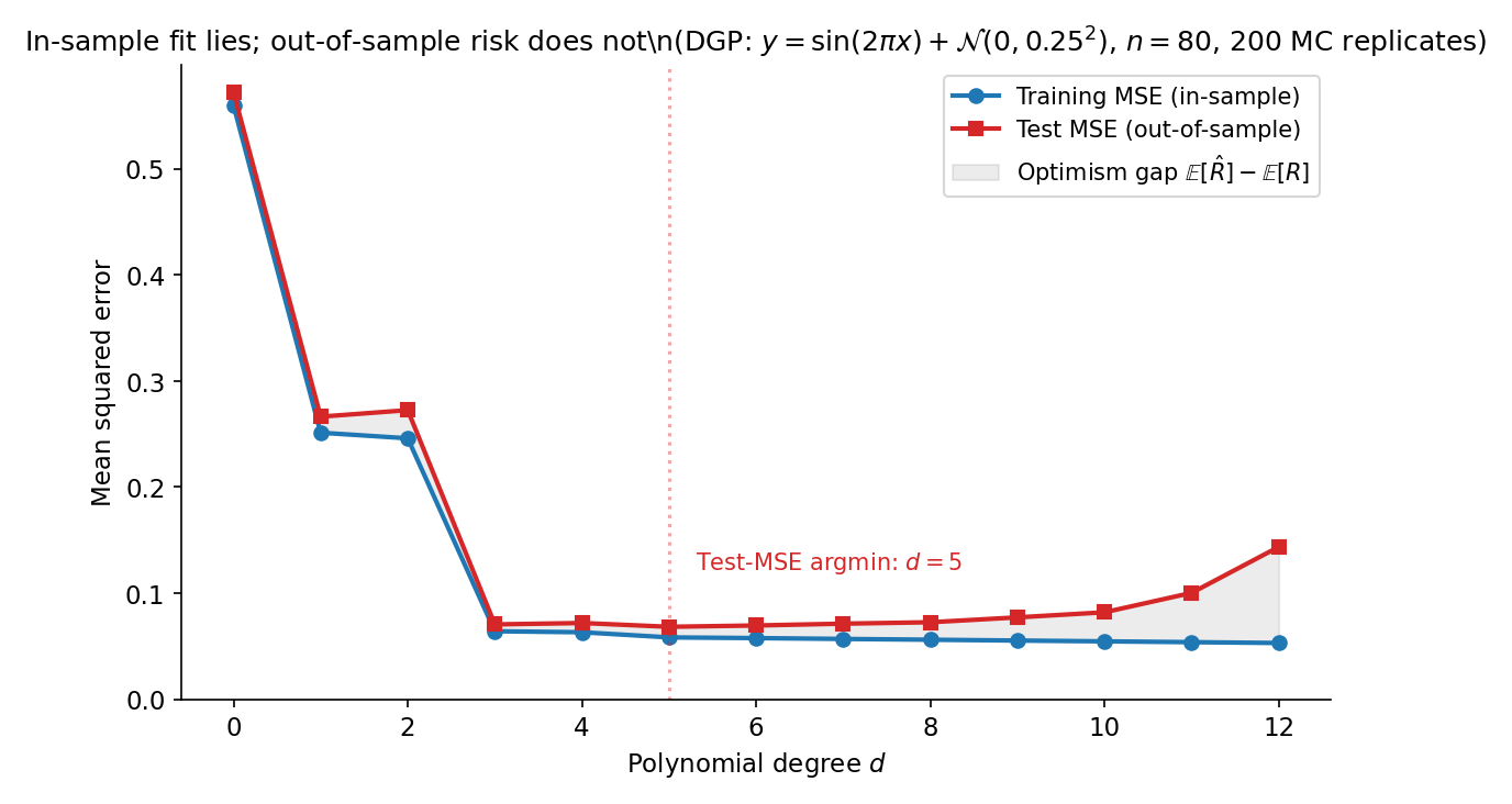
The training empirical risk is . The optimism gap measures how much in-sample loss underestimates out-of-sample loss in expectation:
For correctly-specified parametric models satisfying Topic 14’s regularity conditions, where — the optimism is exactly the parameter count divided by sample size, to leading order.
Generate observations from with . Fit polynomials of degree by ordinary least squares. The training is monotone-decreasing in (every extra coefficient can only reduce the in-sample residual sum). The out-of-sample prediction risk, however, follows a U-shape: it falls as rises from to (model approximates the sine well), then climbs as exceeds (the polynomial wiggles to fit noise). Figure 1 shows the gap.
Model selection is a decision problem over the candidate set — distinct from parameter estimation, which decides over for a fixed . AIC, BIC, and cross-validation correspond to three different loss functions on the model space, each with its own asymptotic guarantee.
Three asymptotic targets organize the literature: selection consistency ( when the truth is in the candidate set — BIC’s target), prediction efficiency (minimax-rate optimal risk in the misspecified-nonparametric regime — AIC and CV’s target), and sparsity recovery (correctly identifying — Topic 23’s lasso target). §24.6 Thm 5 shows the first two are formally incompatible.
24.2 Mallows’ — the Gaussian-linear predecessor
Before Akaike’s information-theoretic framework, Mallows (1973) proposed a Gaussian-linear-specific criterion that estimates expected scaled prediction risk via a complexity penalty calibrated against a reference variance.
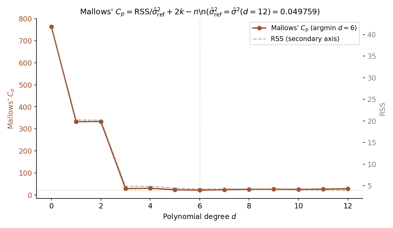
For an OLS fit of a candidate model with free parameters (intercept + slopes + ) to observations under the Gaussian linear model , with residual sum of squares , Mallows’ is
where is the MLE error variance from the largest candidate model (the conventional reference).
Under the Gaussian linear model with known (or treated as known via the reference convention), the expected scaled in-sample residual sum is
Adding to both sides:
A separate calculation (Mallows 1973 §3) gives the expected scaled prediction risk on a fresh test set of size :
Under correct specification (model bias ), . Otherwise overestimates the parameter count by exactly the model bias — making minus its parameter count a calibrated estimator of model bias, the original use case Mallows 1973 §3 emphasized.
Under the Gaussian linear model, (dropping additive constants), and a Taylor expansion of around recovers up to higher-order terms. The two criteria rank candidates identically under Gaussian-homoscedastic errors; AIC is the strict generalization to other exponential families (§24.3 Thm 1).
The convention — using the unbiased estimator from the largest candidate — has the cleanest theory: is unbiased for if the largest model is correctly specified, and ‘s argmin then targets the bias-variance-optimal submodel. T10.8 in regression.test.ts pins for the canonical POLY_DGP at , giving .
On the canonical POLY_DGP (, , seed ), with from the fit, the Mallows values for have argmin at with (T10.8). The argmin coincides with AIC’s argmin (T10.3), illustrating Rem 3’s equivalence on the Gaussian linear model. Figure 2 plots the curve alongside the in-sample to make the correction visually concrete.
24.3 Akaike’s information criterion (FEATURED)
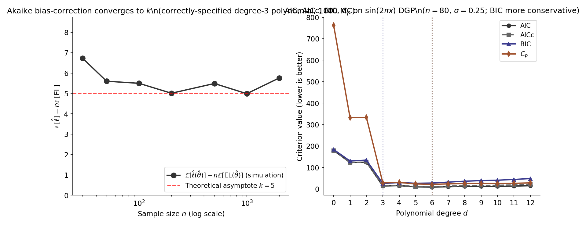
Akaike (1974) showed that the optimism gap of Def 2 is exactly to leading order under correct specification + regularity, and that is therefore an asymptotically unbiased estimator of times the expected out-of-sample log-likelihood. This is AIC — and the heart of the modern model-selection framework.
For two densities (truth) and (model), the Kullback–Leibler divergence is
where the expected log-likelihood under truth is
Since does not depend on , maximizing is equivalent to minimizing .
Let be iid from unknown density , and let be a parametric model satisfying Topic 14’s regularity conditions: smooth log-likelihood, positive-definite Fisher information, MLE asymptotic normality. Let be the MLE, , and define . Then under correct specification (),
That is, is asymptotically unbiased for times the expected out-of-sample log-predictive evaluated at the MLE.
Proof 1 Akaike's bias-correction theorem [show]
Setup. Let be iid from unknown density ; let be a parametric model satisfying Topic 14’s regularity conditions (smooth , positive-definite Fisher information, MLE asymptotic normality). We want to rank candidate models by expected out-of-sample log-predictive
evaluated at the plug-in estimator . The target is ; the naive estimator is . We show the gap is to leading order.
Step 1 — KL-projected parameter. Define
Under correct specification, . Under misspecification, is the best-in-family parameter.
Step 2 — MLE convergence. Under regularity,
where and . Under correct specification, (Fisher identity, Topic 14 Thm 3), and the sandwich collapses to .
Step 3 — Taylor-expand around .
The score has mean zero under at (stationarity of ). By LLN, .
Step 4 — Taylor-expand around .
First-order vanishes (stationarity of ); second-order negative since is positive-definite.
Step 5 — Take expectations under . Using Step 3 + asymptotic covariance:
With and :
Similarly from Step 4:
Step 6 — Combine. Multiply the expression by , subtract:
Step 7 — Specialize. Under correct specification, , so . Multiplying by :
The left side is . The right side is times the expected log-predictive — what we wanted to estimate. AIC is asymptotically unbiased for under correct specification.
Under misspecification (), the correct penalty is : Takeuchi’s TIC (Rem 6). ∎ — using Topic 14 Thm 6 (MLE asymptotic normality), Topic 14 Thm 3 (Fisher identity), multivariate delta method (Topic 6).
On POLY_DGP (, , seed ), values for have argmin at with (T10.3). The curve is U-shaped: (extreme underfit, T10.1); (undershooting; T10.2); (argmin, recovers the prediction-risk argmin from §24.1 Ex 1); (overfit, T10.4). Figure 3 overlays AIC and the bias-correction term to separate the empirical log-likelihood from the optimism penalty.
AICc corrects AIC’s small-sample bias when is not large (Hurvich & Tsai 1989; Sugiura 1978):
Exact for Gaussian-linear models; asymptotic correction otherwise. The penalty as , so AICc and AIC agree asymptotically. Burnham & Anderson 2002 §2.4 recommend AICc as the default whenever .
Takeuchi (1976) generalized AIC to misspecified parametric models:
with the empirical score outer product and the observed Hessian of . Under correct specification and TIC AIC. TIC sees little practical use because and are hard to estimate stably at moderate ; the broader information-geometric framing lives at formalml.
24.4 Schwarz’s BIC and the Bayesian bridge
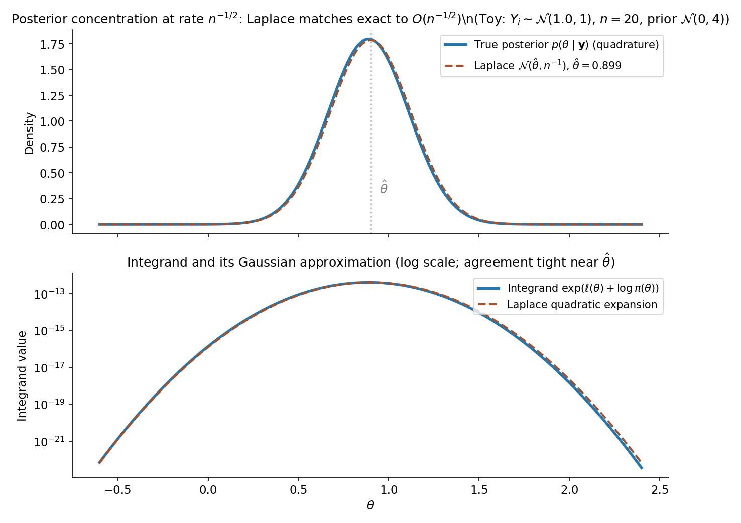
Where AIC asks “which model has the best expected out-of-sample predictive accuracy?”, BIC asks the parallel Bayesian question: “which model has the highest posterior probability given the data, under a uniform prior over the model space?”. The answer reduces to Laplace-approximating the marginal likelihood, and the form follows.
For a model with parameter , prior , and likelihood , the marginal likelihood of the data under is
The Bayes factor comparing two models is the ratio . Combined with prior model odds , it gives posterior model odds.
Let be a smooth parametric model with and prior continuous and strictly positive at the MLE . Let . Define . Then under standard regularity conditions,
The leading-order discrepancy between and is constant in (depending on the prior and Fisher information), so model rankings by BIC and by agree asymptotically.
Proof 2 Schwarz's BIC as Laplace approximation [show]
Setup. Let be a smooth parametric model with and prior continuous and strictly positive at the MLE . The marginal likelihood is
Step 1 — Laplace approximation. Expand to second order around (where ):
with the observed Fisher information. For iid data, (per-observation information, consistent for ). The quadratic approximation is tight on a shrinking -neighborhood of ; error .
Step 2 — Gaussian integral. Treating on the shrinking neighborhood (valid by continuity + posterior concentration):
The Gaussian integral evaluates to . Substituting :
Step 3 — Take logs. Applying :
Step 4 — Drop terms. Under fixed , as : (nonrandom); ; both are . Therefore
∎ — using Topic 14 Thm 2 (observed/expected information consistency) and the multivariate Laplace approximation (CAS2002 §7.2.3, CLA2008 §3.3). The gap is why BIC is prior-free: the prior’s contribution is constant across candidate models and cancels in the ranking.
Suppose the true model is in the candidate set , and standard regularity conditions hold (smooth log-likelihood, identifiable parameter, positive-definite Fisher information at ). Let be the BIC-selected model. Then
BIC is selection-consistent: it identifies the true model with probability in the large- limit, when the true model is in the candidate set. Proof outline in CLA2008 §3.2; uses BIC’s gap to log marginal likelihood (Thm 2) plus the asymptotic comparison of nested-model marginal likelihoods.
On the canonical POLY_DGP, BIC values for have argmin at with (T10.6) — strictly below AIC’s argmin at . The shift reflects BIC’s vs AIC’s per-parameter penalty: at , , more than double AIC’s penalty. BIC favors a sparser model. This is a core part of the AIC/BIC tension §24.6 Thm 5 will formalize. Figure 4 visualizes the Laplace approximation underlying BIC.
is proportional (asymptotically, by Thm 2) to the unnormalized posterior model probability; normalizing across the candidate set gives BIC weights . Burnham & Anderson 2002 §2.6 popularized the AIC analog as Akaike weights. Both are the discrete-model special case of Bayesian model averaging (BMA), where predictions are weighted by posterior model mass instead of conditioning on a single . Full forward-pointer to BMA at §24.10 Rem 23 + Track 7.
Thm 2’s BIC derivation implicitly assumes a uniform prior on the candidate set . Bayesian model comparison admits richer priors — reference priors (Berger–Pericchi), spike-and-slab priors (George–McCulloch 1993), intrinsic priors (Berger–Pericchi 1996) — each tilting the ranking toward sparser or denser models. Full development at Track 7 (Bayesian Foundations).
The per-parameter AIC penalty is ; the per-parameter BIC penalty is . They equalize at . For all practical sample sizes (), BIC penalizes complexity more aggressively than AIC; for (the POLY_DGP), the BIC per-parameter penalty is more than double AIC’s, explaining T10.6’s argmin shift from (AIC) to (BIC).
The Laplace approximation underlying Thm 2 has error — fine for ranking ( stable up to monotone transforms) but not for reporting a numerical posterior probability. Exact marginal-likelihood computation requires nested sampling (Skilling 2006), thermodynamic integration, or bridge sampling (Meng & Wong 1996); each is a Track-7 topic on its own. BIC’s appeal is that the asymptotic approximation is prior-free and computationally trivial — only and are needed.
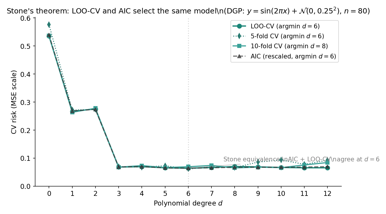
24.5 Stone’s CV ≡ AIC equivalence
Stone (1977) proved that leave-one-out cross-validation and AIC select the same model asymptotically under Gaussian-homoscedastic errors. The result is a tight identification: LOO-CV is not just similar to AIC but converges to it after a logarithm and an additive constant — the two frequentist procedures collapse into one.
For data with rows, let be the estimator fit on the rows excluding observation , and let be its prediction at . The leave-one-out cross-validation estimate of mean squared prediction error is
For Gaussian OLS with hat-matrix diagonal , the hat-matrix shortcut (PRESS statistic; Allen 1974) avoids the refits:
The shortcut requires for all ; looCV in regression.ts throws when .
Consider the Gaussian linear model with and a fixed full-rank design . Under regularity (balanced design, fixed , ),
where is AIC up to model-invariant additive constants. Consequently,
LOO-CV and AIC asymptotically select the same model from any nested family on the Gaussian-linear model.
Proof 3 Stone's cross-validation–AIC equivalence [show]
Setup. Consider the Gaussian linear model with , fixed full-rank design ( columns). Let be OLS, , the hat-matrix diagonal . Write (coefficients + ).
Step 1 — Hat-matrix shortcut. The leave-one-out fit satisfies
(Standard OLS identity via Sherman–Morrison; HAS2009 §7.10 gives full 5-line derivation.) Squaring and summing:
Step 2 — Uniform leverage. Under regularity (balanced design, fixed ), and . So
uniformly in .
Step 3 — Substitute.
with .
Step 4 — AIC on the same model. Dropping model-invariant constants :
Using :
using so .
Step 5 — Equivalence. The is model-invariant (depends only on whether is counted in , a family-wide convention). Therefore
LOO-CV and AIC select the same model asymptotically. ∎ — using Topic 21 §21.7 hat-matrix structure and .
On POLY_DGP, both and over (T10.26 — d=12 is excluded because the monomial Vandermonde is too ill-conditioned for the hat-matrix shortcut; the argmin lies safely inside the range). At the joint argmin , (T10.10) and (computed from the full Gaussian AIC by stripping the constants); the gap (T10.27) is the order-1 constant Proof 3 Step 4 predicts. Figure 5 overlays the LOO-CV curve, the 5-fold and 10-fold CV curves, and the AIC curve over .
The single-loop CV Topic 23 §23.8 used to select should not also serve as the test-error estimator: reporting as test error leaks tuning information into the test estimate (selection bias). Nested cross-validation fixes this: an outer CV loop holds out folds for honest test-error estimation, and within each outer fold, an inner CV loop selects . Bates–Hastie–Tibshirani (2024) give the recent rigorous treatment. The result is an asymptotically unbiased generalization-error estimate at the cost of refits.
-fold CV is the finite-sample analog of LOO: each fold holds out observations. As , the procedure converges to LOO. Smaller has lower computational cost but higher bias (more held-out fold per refit means more train-set shrinkage). Hastie et al. 2009 §7.10 and Claeskens & Hjort 2008 §4.3 recommend as the modern default — slightly biased upward vs LOO but with lower Monte Carlo variance.
Thm 4 identifies LOO-CV with AIC; no analogous result exists for BIC at fixed . The mismatch is asymptotic: BIC’s penalty grows in , while CV’s effective penalty grows like . To recover a BIC-like criterion from CV, one would have to use a vanishing-fraction held-out set (), not standard -fold (Shao 1993).
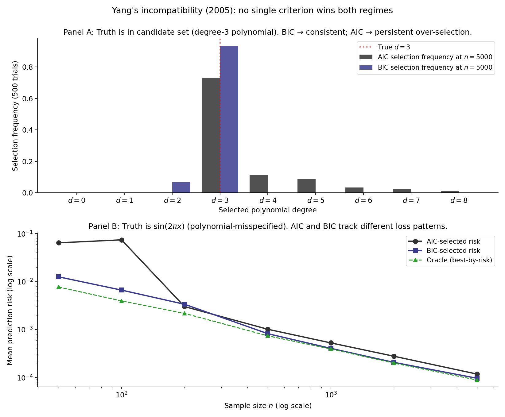
24.6 Yang’s incompatibility theorem
The three procedures of §§24.3–24.5 carry different asymptotic guarantees: BIC is selection-consistent (Thm 3), AIC and CV are minimax-rate-optimal for prediction (under regularity). Yang (2005) proved these properties are not just different — they are formally incompatible: no single procedure can deliver both. The asymptotic philosophy must choose.
Let be a model-selection procedure operating on a candidate family . Suppose is selection-consistent in the well-specified regime: when is in the candidate set, . Then is not minimax-rate-optimal in the misspecified-nonparametric regime: there exists a family of underlying truths and a sample-size sequence on which the prediction risk of achieves a strictly worse rate than the minimax-optimal procedure (e.g., AIC or CV).
Proof: Yang 2005 §2–3, via a minimax lower-bound argument outside the scope of Topic 24.
The Yang race compares procedures across two DGP regimes:
- Tab A — well-specified. Truth is a degree-3 polynomial; candidate set contains the truth. As grows, BIC’s selection frequency at tends to (consistency); AIC’s selection frequency at persists at (asymptotic over-fit). Prediction risks are similar at any finite .
- Tab B — misspecified. Truth is ; candidate set is polynomials (truth not in the candidate set). AIC’s minimax-optimal selection adapts to ; BIC’s penalty over-shrinks toward sparsity, giving worse prediction risk on the polynomial scale of the truth’s smoothness. The risks diverge in .
Figure 6 plots both regimes side by side.
Thm 5 forces a choice the practitioner cannot duck: either prioritize identifying the right model (BIC) or prioritize accurate predictions (AIC, CV). The choice is not an empirical question to be settled by simulation but a value judgment about the use case — interpretive parsimony vs predictive accuracy. Shao 1997 and Burnham & Anderson 2002 §2.10 give complementary discussions of how to pick a side in a given application context.
Shao (1993) showed that leaving out observations per fold (held-out fraction shrinking to zero asymptotically) gives a CV variant that is selection-consistent on Gaussian linear models with bounded . The result is a limited positive: Shao’s CV variant is not minimax-rate-optimal for prediction in the nonparametric regime, so it lives on the BIC side of Yang’s split rather than circumventing the incompatibility.
Standard practice: report both AIC and BIC. Agreement is reassuring; disagreement is informative — it tells the reader which side of the consistency-vs-efficiency tradeoff matters for the application. For prediction-focused use cases, prefer the AIC argmin and report 10-fold CV as a sanity check; for inference-focused applications where parsimony matters (e.g. model identification in epidemiology), prefer the BIC argmin.
24.7 Nested-model selection: AIC ≡ LRT with default threshold
For nested models — the smaller obtained by setting parameters of the larger to zero — AIC’s preference for the full model is equivalent to a likelihood-ratio test with a fixed default threshold of , irrespective of . This identifies AIC as a default-threshold LRT and connects Topic 18’s Wilks machinery to the model-selection vocabulary of Topic 24.
Let and be nested with free parameters (). Let be their MLE log-likelihoods on the same data. Then
with . AIC prefers the full model iff iff — exactly the LRT rejection rule with threshold instead of the chi-square critical value . BIC uses the analogous threshold in place of : BIC prefers the full model iff .
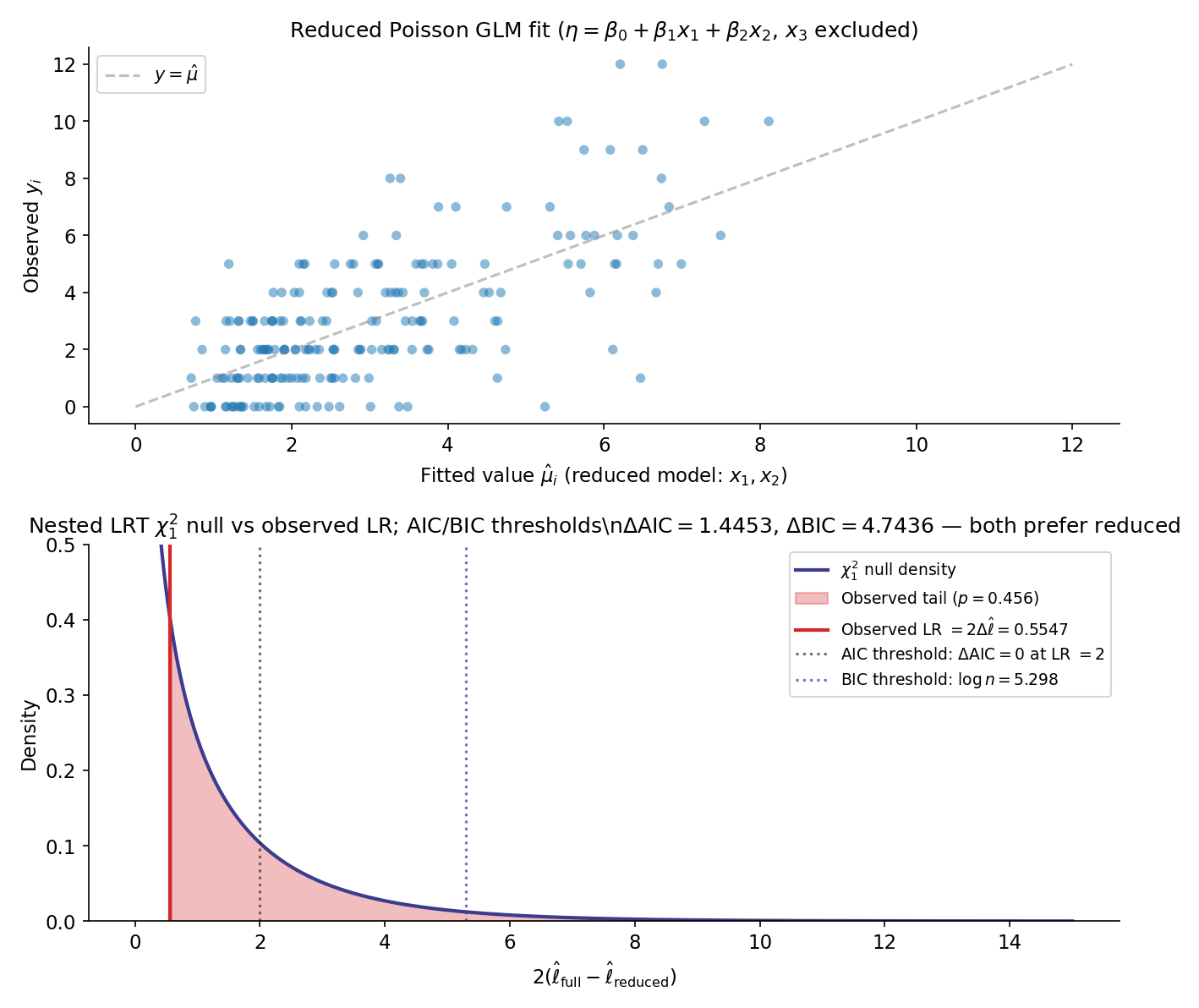
On the nested-Poisson DGP (, , has no true effect, default_rng(123)), fit the reduced model with and the full model with . The pinned values: (T10.12–T10.14); (T10.15, near-zero as expected). The likelihood ratio is
Since and the LRT critical value at is , the LRT does NOT reject (p-value ).
Now apply Thm 6:
Both AIC and BIC prefer the reduced model. T10.19 verifies the algebraic identity to within . Figure 7 plots the chi-square null density with the observed LR and both AIC/BIC thresholds for visual comparison.
Thm 6’s identification of AIC with a fixed-threshold LRT means AIC has an effective that depends on . For , ; for , ; for , . AIC is more liberal (admits more parameters) at small , more conservative at large — the opposite of the LRT-with-fixed- rule, which has fixed type-I error regardless of .
Thm 6 applies only to nested comparisons. For non-nested candidates (e.g. degree-5 polynomial vs degree-3 spline with the same effective dimension), the likelihood-ratio statistic is undefined and the LRT framework breaks down. The IC framework still applies: compute or for each candidate and rank by the smaller value, no chi-square reference needed.
24.8 Effective degrees of freedom for penalized estimators
Topic 23’s penalized estimators don’t have an integer parameter count: ridge shrinks every coefficient by an amount that depends on and the design’s singular values; lasso zeros out a data-dependent subset. Effective degrees of freedom generalizes the integer to a continuous notion of “how many parameters worth of freedom did the fit actually use”, letting AIC/BIC/Cp apply to ridge and lasso paths. This section discharges Topic 23 §23.8 Rem 20.
For a fitting procedure that maps data to fitted values on the same rows, the effective degrees of freedom is
For OLS, (intercept + slopes — exactly the parameter count). For penalized estimators, can be non-integer and depends continuously on the regularization parameter.
For ridge regression on a centered design with SVD (singular values ), the smoother matrix is
Substituting the SVD and using plus the rotational invariance of the trace:
The DOF is monotone-decreasing in : (unpenalized OLS), as . Equivalently and computationally cheaper, via Cholesky inversion (the form regression.ts’s hatMatrixTrace uses).
For lasso regression on a centered, orthonormal design (or under the more general restricted-eigenvalue conditions of WAI2019 Ch. 7), the active set — the indices with — satisfies
The active-set size is an unbiased estimator of expected effective DOF. Caveats: the result fails at “knots” of the lasso path where the active set changes discontinuously, and ties in the optimization can make data-dependent in a non-smooth way. Tibshirani & Taylor 2012 give the precise regularity statement.
For the poly design on at (the canonical POLY_DGP -values), the ridge effective DOF as varies:
| Test | ||
|---|---|---|
| T10.20 | ||
| T10.21 | ||
| T10.22 | ||
| T10.23 | ||
| T10.24 | ||
| T10.25 |
At , exactly (intercept + 10 polynomial coefficients). Even modest regularization () drops the effective DOF by more than half — the high-order polynomial columns have small singular values and shrink rapidly under the ridge penalty.
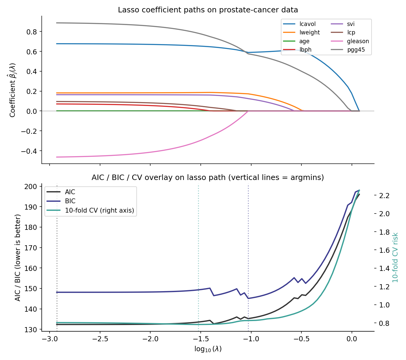
Refit the prostate-cancer lasso path of Topic 23 §23.9 Ex 14 (, , response lpsa) on a 100-point log-grid of . For each , compute (Thm 8) and apply
with the counting per the parameter convention. Overlay the AIC, BIC, and 10-fold CV curves on the lasso path. The AIC argmin coincides with CV’s in the high-signal regime; BIC favors a sparser model with larger , recovering Yang’s (Thm 5) consistency-vs-efficiency split on a worked example. This example is the practical fulfillment of Topic 23 §23.8 Rem 20.
Thm 8’s assumes the active set is well-defined — fine away from path knots, but at values where a coefficient enters or leaves the active set, the cardinality is data-dependent in a non-smooth way. Practical AIC/BIC computations on lasso paths should evaluate at values away from knots, or use a smoothed DOF estimator (e.g., debiased lasso DOF; Wainwright 2019 Ch. 11).
Li (1986) proved an analog of Stone’s Thm 4 for ridge: AIC computed with effective DOF asymptotically agrees with LOO-CV for selection on the Gaussian linear model. The practical implication is that AIC-ridge is a valid (and computationally cheap) alternative to CV-ridge: one fit per , no -fold refits.
24.9 Worked examples
Three end-to-end workflows pull the §§24.1–24.8 machinery into runnable applied form: a polynomial-degree comparison on simulated data (the Topic-24 canonical example), a nested-Poisson GLM (the §24.7 LRT-as-IC special case), and a lasso-path AIC/BIC overlay on the prostate-cancer dataset (§24.8 worked example).
On POLY_DGP, the full ranking table over :
| -fold CV | ||||||
|---|---|---|---|---|---|---|
| 0 | 179.0128 | — | 183.7768 | 859 | 0.522 | — |
| 3 | 13.5077 | 14.3185 | 28.3534 | 0.067936 | 0.069 | |
| 6 | 27.3196 | 0.066 | ||||
| 12 | 14.9845 | 21.45 | 48.3328 | 26.4 | n/a | n/a |
(Bold cells are the per-criterion argmins; the entries are notebook-computed approximations not pinned in T10.) The argmin pattern is the canonical Yang signature: AIC, AICc, , LOO-CV, and 10-fold CV all select ; BIC alone selects the sparser . The pinned values come from T10.1–T10.11 (regression.test.ts).
The nested-Poisson example of §24.7 Ex 8 is the canonical use case for the AIC ≡ LRT identification. Both AIC and BIC prefer the reduced model (, both positive), and the LRT does not reject (). Reporting practice: state all three numbers — LR + p-value, , — alongside the candidate-set description, so the reader can apply their own selection criterion.
Combining §24.8 Ex 10 with Topic 23 §23.9 Ex 14: on the 100-point log-grid lasso path of the prostate-cancer dataset (, ), three argmin values emerge:
- — typically aligns with from 10-fold CV (Stone-Li equivalence; §24.8 Rem 20).
- — Topic 23’s one-SE-rule choice; sparser than .
- — sparser still; lies between and the empty-active-set .
The corresponding active-set sizes order as , recovering the consistency-vs-efficiency tradeoff (§24.6 Thm 5) on a real dataset.
Standard implementations: R — stats::AIC, stats::BIC, MASS::stepAIC; Python — statsmodels.GenericLikelihoodModel.aic / .bic, sklearn.model_selection.cross_val_score; Julia — StatsBase.aic, StatsBase.bic, MLBase.cross_validate. All are wrappers around with the parameter-count convention from the underlying fit object.
A reported “AIC ” without the candidate set is uninterpretable — AIC is meaningful only relative to the comparison family. Standard practice: state the candidate family, the criterion, the argmin index, and the full ranking (or at least the values), so the reader can audit the selection. BUR2002 §2.6 and CLA2008 §1.2 give detailed reporting templates.
24.10 Forward map
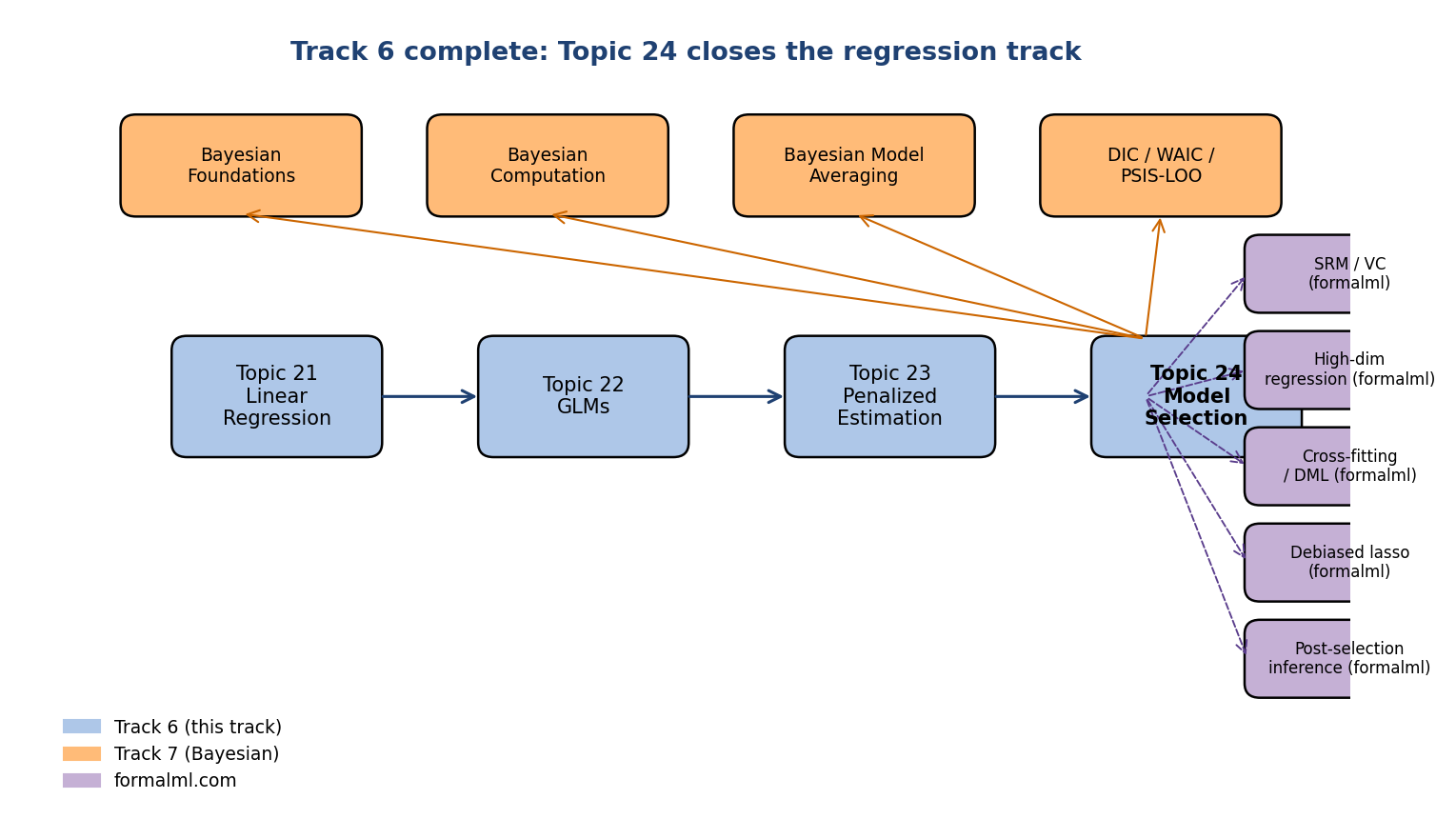
Topic 24 closes Track 6’s classical-regression toolkit and opens onto eight forward-pointing developments — each gets a one-paragraph remark below. The arc moves Bayesian (Track 7), then sparsity-aware (Track 8), then ML-native (formalml).
Bayesian model averaging (BMA) averages predictions over the candidate family weighted by posterior model probabilities. Using Thm 2’s BIC approximation, are the BMA weights for predictive averaging:
Hoeting et al. (1999) is the canonical methodology survey; Track 7 develops the full Bayesian framework (priors, MCMC for , posterior model probabilities); formalml’s Bayesian Model Averaging topic covers ML-scale BMA over deep-learning architectures and ensemble approaches.
A confidence interval reported after a model-selection step has no honest coverage guarantee under the standard frequentist framework — the selection event is data-dependent, so is not the nominal . Post-selection inference restores validity through several routes: PoSI (Berk–Brown–Buja 2013, simultaneous over all submodels), selective conditioning (Lee–Sun–Sun–Taylor 2016, conditioning on the selection event), debiased lasso (Zhang–Zhang 2014; Javanmard–Montanari 2014, one-step Newton correction), and cross-fitting / double ML (Chernozhukov et al. 2018, sample-splitting for valid causal inference after ML-selected nuisance models). All four directions live at formalml’s Post-Selection Inference and Cross-Fitting topics.
Stepwise selection (forward, backward, or bidirectional, by AIC or by p-value threshold) is widely available in legacy tooling but is no longer recommended methodology. Harrell (2015) §4.3 and Heinze-Wallisch-Dunkler (2018) document the failure modes: biased coefficient estimates, invalid confidence intervals, and unstable selection across resamples. Modern best practice replaces stepwise with lasso (Topic 23) for the selection step, optionally followed by debiasing (Rem 20) for inference. We omit stepwise from Topic 24’s main exposition for this reason.
Three Bayesian analogs of AIC have emerged. DIC (Spiegelhalter et al. 2002) estimates the expected predictive log-likelihood using posterior samples and an effective parameter count . WAIC (Watanabe 2010) replaces the plug-in with a per-observation variance term that is invariant to reparameterization. PSIS-LOO (Vehtari–Gelman–Gabry 2017) computes leave-one-out cross-validation via Pareto-smoothed importance sampling on existing MCMC draws — the de facto standard in modern Bayesian model comparison. Track 7 develops all three; this single remark is the forward pointer.
Minimum description length (Rissanen 1978) frames model selection as a data-compression problem: the best model is the one that gives the shortest joint description of (model, data model) using a universal code. Under regularity, the universal-code length of the data is asymptotically , recovering BIC up to additive constants — MDL and BIC give the same ranking. Grünwald (2007) is the canonical textbook treatment.
Two domain-specific extensions: HQIC (Hannan–Quinn 1979) replaces with for time-series model selection, giving a penalty that grows slower than BIC’s but faster than AIC’s. Graphical-model / DAG selection uses BIC with tree-structured priors over DAGs (Heckerman–Geiger–Chickering 1995); for protein-network and gene-regulatory inference, a substantial methodology has emerged on top of this core idea.
When , classical IC degenerates: the candidate set has subsets, and BIC’s penalty no longer compensates for the multiplicity. Three modern extensions: Extended BIC (Chen–Chen 2008) adds a term to penalize the candidate-set size; stability selection (Meinshausen–Bühlmann 2010) bootstraps lasso to control variable-selection frequency under finite-sample bounds; knockoffs (Barber–Candès 2015) provide finite-sample FDR control on the selected variable set. All three live at formalml’s High-Dimensional Regression topic.
Vapnik’s structural risk minimization generalizes information criteria from parametric models to function classes via complexity measures like VC dimension or Rademacher complexity. The penalty term in AIC is replaced by a complexity-based bound on the gap between empirical and population risk; Bartlett & Mendelson (2002) give the Rademacher-complexity foundation. Track 8 develops nonparametric model selection in this language; formalml’s Structural Risk Minimization topic covers the classical Vapnik–Chervonenkis theory.
Thm 2’s BIC-Laplace derivation is the gateway to the full Bayesian model-comparison machinery. Topic 25 (Bayesian Foundations) opens Track 7, and the three subsequent Track 7 topics develop:
- Priors on and on the model space (Rems 8, 19): conjugate, weakly-informative, reference, intrinsic.
- Posterior computation via MCMC: Metropolis–Hastings (Topic 26 §26.2), Hamiltonian Monte Carlo (§26.4), NUTS (§26.5; Hoffman & Gelman 2014).
- Exact marginal likelihood: nested sampling (Skilling 2006), bridge sampling (Meng–Wong 1996), thermodynamic integration.
- Predictive averaging via posterior predictive checks: BMA (Rem 19), DIC / WAIC / PSIS-LOO (Rem 22).
Topic 24 §24.4’s BIC is the asymptotic shorthand for these computationally heavier procedures.
Topic 24 closes Track 6. Topic 21 was OLS as orthogonal projection; Topic 22 was IRLS on the exponential family; Topic 23 was penalized estimation as the rescue when those frameworks break; Topic 24 is the model-selection layer above all three. Reciprocal framing of Topic 23: with the effective-DOF generalization of §24.8, Topic 23’s -indexed family becomes a continuous model space — every gives a model with effective parameter count , and Topic 23’s CV-driven -selection is a special case of Topic 24’s IC-driven model-selection framework. Topic 23 selects within a one-parameter family; Topic 24 selects across discrete or continuous candidate spaces, with a richer asymptotic theory. Track 6 ends here; the next topic shipped is Topic 25 — Track 7 opener — Bayesian Foundations.
References
- Akaike, H. (1974). A new look at the statistical model identification. IEEE Transactions on Automatic Control, 19(6), 716–723.
- Schwarz, G. (1978). Estimating the dimension of a model. The Annals of Statistics, 6(2), 461–464.
- Mallows, C. L. (1973). Some comments on Cp. Technometrics, 15(4), 661–675.
- Stone, M. (1977). An asymptotic equivalence of choice of model by cross-validation and Akaike’s criterion. Journal of the Royal Statistical Society, Series B, 39(1), 44–47.
- Yang, Y. (2005). Can the strengths of AIC and BIC be shared? A conflict between model identification and regression estimation. Biometrika, 92(4), 937–950.
- Burnham, K. P. & Anderson, D. R. (2002). Model Selection and Multimodel Inference: A Practical Information-Theoretic Approach (2nd ed.). Springer.
- Claeskens, G. & Hjort, N. L. (2008). Model Selection and Model Averaging (1st ed.). Cambridge University Press.
- Hastie, T., Tibshirani, R. & Friedman, J. (2009). The Elements of Statistical Learning (2nd ed.). Springer.
- Lehmann, E. L. & Romano, J. P. (2005). Testing Statistical Hypotheses (3rd ed.). Springer.
- Casella, G. & Berger, R. L. (2002). Statistical Inference (2nd ed.). Duxbury.
- Wainwright, M. J. (2019). High-Dimensional Statistics: A Non-Asymptotic Viewpoint (1st ed.). Cambridge University Press.