Likelihood-Ratio Tests & Neyman-Pearson
Optimality theory — Neyman-Pearson's lemma, Karlin-Rubin UMP construction, Wilks' χ² theorem, and the first-order equivalence of Wald, Score, and LRT.
18.1 From Framework to Optimality
Two tests have the same size. Both reject the null 5% of the time when the null is true. One rejects a true effect of size with probability ; the other rejects with probability . Which should we use? Topic 17 built a framework for valid testing but left this question open. This topic answers it: we characterize when a uniformly most powerful test exists (Neyman-Pearson, Karlin-Rubin), construct the likelihood-ratio test as a general-purpose procedure when it doesn’t, and prove that the three asymptotic tests — Wald, Score, LRT — agree to first order under the null.
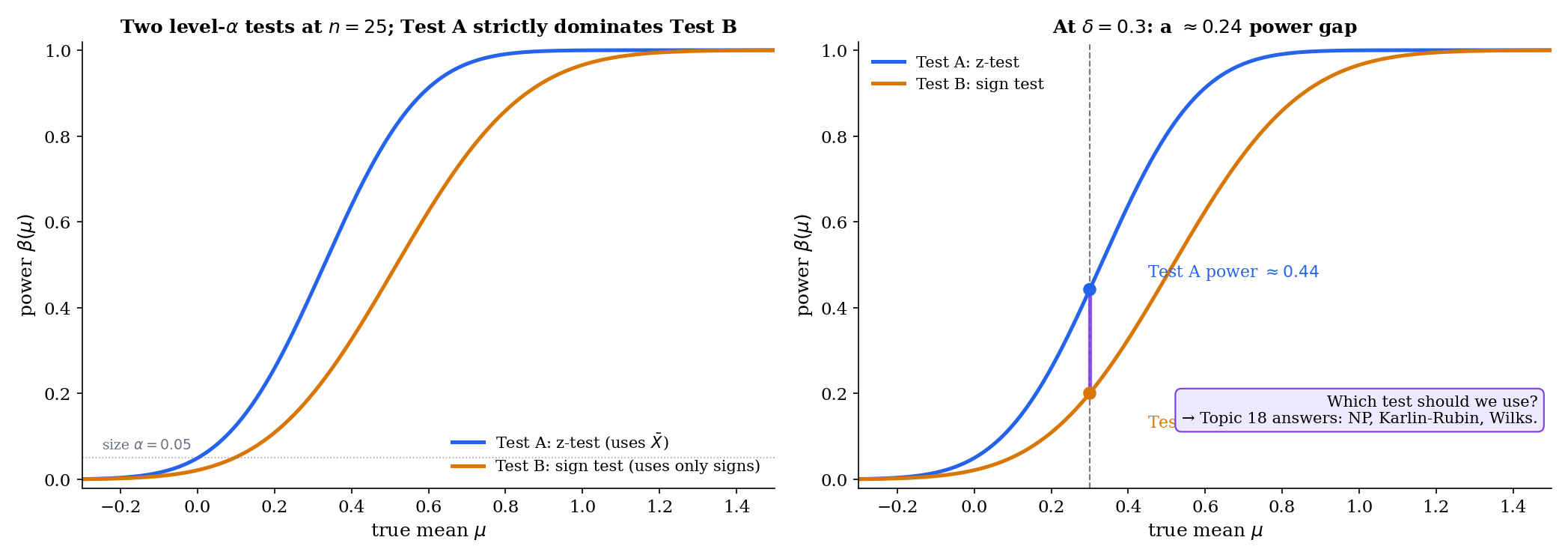
A level- test is valid if its Type I error is at most . That is not a hard standard to meet. The trivial “reject with probability regardless of data” test is valid — and has power exactly at every alternative. Every test we wrote down in Topic 17 (z-test, t-test, variance test, binomial exact) is valid for its parametric family. But validity does not single out which level- test to use.
Optimality asks the harder question: among all valid level- tests, which maximizes power? The answer depends on whether the hypotheses are simple or composite and on the structural geometry of the likelihood family. Where the answer exists — NP lemma, Karlin-Rubin — it is a uniqueness result, not merely an existence one. Where it does not — two-sided composite alternatives in most families — the LRT is the best general-purpose substitute, and we pay a price for that generality in the form of asymptotic rather than finite-sample optimality.
Topic 18 is built around four results. The first two hold at every sample size; the last two are asymptotic.
-
Neyman-Pearson lemma (§18.2). Simple-vs-simple optimality via a three-step indicator-function argument. Provable from integration alone — no convergence theory required.
-
Karlin-Rubin theorem (§18.3). One-sided composite optimality via monotone likelihood ratio (MLR), using the NP lemma as an internal engine. The MLR families are exactly where “one test is most powerful at every alternative simultaneously” — i.e., UMP — becomes possible.
-
Wilks’ theorem (§18.6). The composite LRT’s null distribution converges: where is the number of parameter restrictions. Proved in 8 steps via Taylor expansion around , remainder control, observed-information-to-Fisher-information, and MLE asymptotic normality (Topic 14 Thm 14.3).
-
Three-tests equivalence (§18.7). Wald, Score, and LRT differ by under . All three collapse to the same quadratic form at leading order. §18.8 quantifies the finite-sample divergence the hides.
The residual sections then extend the theory in specific directions. §18.4 catalogues UMP tests in action; §18.5 formalizes the composite LRT; §18.8 proves reparameterization invariance; §18.9 characterizes local power via non-central ; §18.10 points to the scope boundaries.
Every proof in Topic 18 is written for scalar . Vector- extensions — -df Wilks, UMP unbiased, Hunt-Stein invariance, Chernoff 1954 boundary cases — are stated with pointers to Lehmann-Romano (LEH2005) and nothing more. This is not pedagogical convenience; it is a deliberate scope decision. The scalar case captures every main idea (the pointwise LR comparison of Proof 1, the MLR-yields-UMP argument of Proof 2, the quadratic-approximation of Proof 3). The vector generalizations are mostly bookkeeping — matrix inverses in place of scalar divisions, quadratic forms in place of , and a limit in place of . Readers who need the vector results in production should consult LEH2005 Ch. 3 (vector UMP), Ch. 6 (invariance), and Ch. 12 (large-sample theory). Topic 19 and Topic 20 extend Track 5 with CI duality and multiple testing; vector- extensions to Wilks reappear organically in GLM inference on formalml.com/generalized-linear-models.
18.2 The Neyman-Pearson Lemma
Start with the cleanest case: both and are single points in parameter space. Is there a level- test whose power at exceeds the power of every other level- test? Yes, and the answer is the likelihood-ratio test.
A test (where is the probability of rejecting at observation ) is most powerful (MP) at level against if
That is, maximizes the power at among all tests of size at most . The maximum need not be unique on the boundary of the constraint; uniqueness holds in the interior.
For simple vs simple , the likelihood ratio at observation is
For iid data with density , the LR factorizes: , and we typically work with for numerical stability.
The above is distinct from the composite generalized likelihood ratio defined in Topic 17 §17.9 Def 15. The simple-vs-simple LR compares two specific parameter values; the composite compares the best null fit to the best full-model fit. They coincide when both hypotheses are singletons. §18.5 reintroduces the composite , and §18.6 proves its asymptotic limit.
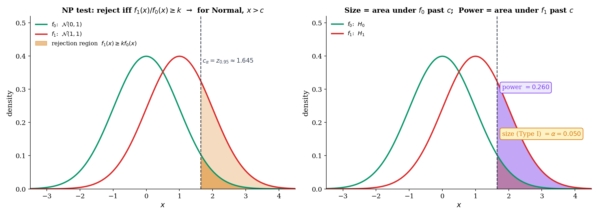
Let have density with respect to a common -finite measure . For testing simple vs simple , fix and let be a threshold. The Neyman-Pearson test
with randomization on the boundary chosen to make , is most powerful level- among all tests with .
Proof [show]
Let be any test with . We prove .
Step 1 — pointwise inequality. For every ,
At any with , we have , so both factors are . At any with , we have , so both factors are . On the boundary the second factor is zero and the inequality holds trivially. Either way, the product is non-negative pointwise.
Step 2 — integrate. Integrating the pointwise inequality against :
Expanding the product and converting integrals to expectations,
Step 3 — apply the size constraint. By construction, . By assumption, . So
Multiplying by preserves the inequality:
i.e., has power at least as large as any other level- test.
∎ — using NEY1933
Let be iid Bernoulli. Test vs with . The likelihood ratio at is
which is monotone increasing in (since implies and ). The NP test rejects iff for some threshold ; randomization at achieves exact size .
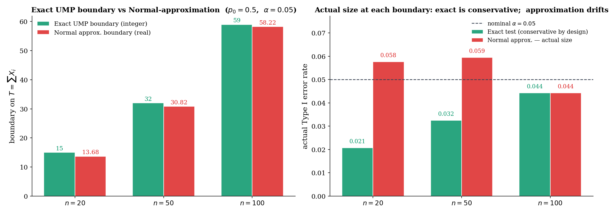
Concretely: for , , , , the NP test rejects at with exact size (the conservative size of §18.4). Power at : (verified in binomialExactPower of Topic 17’s testing.ts).
Let be iid with known. Test vs with . The log-likelihood ratio is
monotone increasing in . The NP test rejects iff for , where is the standard-Normal -quantile. The threshold depends on and and — but not on . The same test is NP against every . That is the geometric seed of the Karlin-Rubin theorem in §18.3.
Numerical check: , , , , . Then , matching npCriticalValue('normal-mean-known-sigma', 0, 1, 25, 0.05, 1) in testing.ts.
Let be iid Exponential with density on . Test vs . The log-likelihood ratio is
If (faster rate, shorter expected waits), the LR is decreasing in : short totals favor . The NP test rejects iff . Under , ; using we get the exact size at .
The direction reversal — shorter totals trigger rejection of “the slower rate is true” — is a common pitfall in exponential-reliability testing. npCriticalValue('exponential', ...) in Topic 17’s testing.ts handles the direction via an explicit Tform label noting the side.
The NP test’s “randomize on the boundary” clause looks strange but is needed only when — i.e., when the test statistic is discrete and falls on an atom. For continuous tests (Normal, Exponential), the boundary has measure zero and no randomization is needed; the size is exactly by choice of . For discrete tests (Bernoulli, Poisson), the exact size without randomization is usually strictly less than — the conservative size of §17.3 Thm 1 and §17.6 Ex 11. We treat randomization as a theoretical device: in practice we rarely implement it, accepting the conservative size in exchange for interpretability.
Theorem 1 is a template — given the two parameter values and a chosen , it tells you what the MP test looks like. It does not by itself produce a usable test of a practical hypothesis like “is this drug better than placebo?” because practical hypotheses are rarely simple-vs-simple. The real is usually composite (“some positive effect of unspecified size”), and the MP test depends on which specific alternative you face. §18.3 asks: when is the NP rejection region the same for every alternative in a composite ? That is the MLR / Karlin-Rubin story.
18.3 Monotone Likelihood Ratio & Karlin-Rubin
The NP test at Example 2 had a remarkable property: the rejection region did not depend on — only on , , , . The same test was NP against every . That property has a name: uniformly most powerful (UMP). Which families give it?
A family has monotone likelihood ratio in if there exists a statistic such that for every pair in , the ratio
Equivalently, is a non-decreasing function of .
A level- test is uniformly most powerful (UMP) against a composite alternative if it is MP level- at every simultaneously. In symbols: for every and every level- test ,
UMP existence is a strong statement — the same rejection region beats every competitor at every alternative.
Let have MLR in . For testing
there exists a threshold (possibly with randomization at for discrete ) such that the test
has size exactly and is UMP level-.
Proof [show]
We prove two things: (i) has size over the composite null , achieving at ; (ii) is MP at every .
Step 1 — size over the composite null. By MLR, for any ,
Consider the NP test (Theorem 1) of the simple ” vs ” with rejection region , which by MLR coincides with for an appropriate depending on . The NP lemma says this test maximizes subject to . Inverting: the power at of any level- test at is bounded by the power at of the NP test at , which is exactly the size at required to achieve size at . Because the rejection region is of NP form with size at , its size at cannot exceed :
Size is maximized at and equals on the composite null boundary.
Step 2 — MP at each . Fix . By MLR,
There exists a threshold such that (same as Step 1, since both are calibrated to size at ). By Theorem 1, the test is MP level- for ” vs ” — and the rejection region does not depend on . The same test is MP at every simultaneously.
Combining Steps 1 and 2: has size on the composite null (achieved at ) and is MP at every alternative. This is the definition of UMP.
∎ — using KAR1956 and Theorem 1
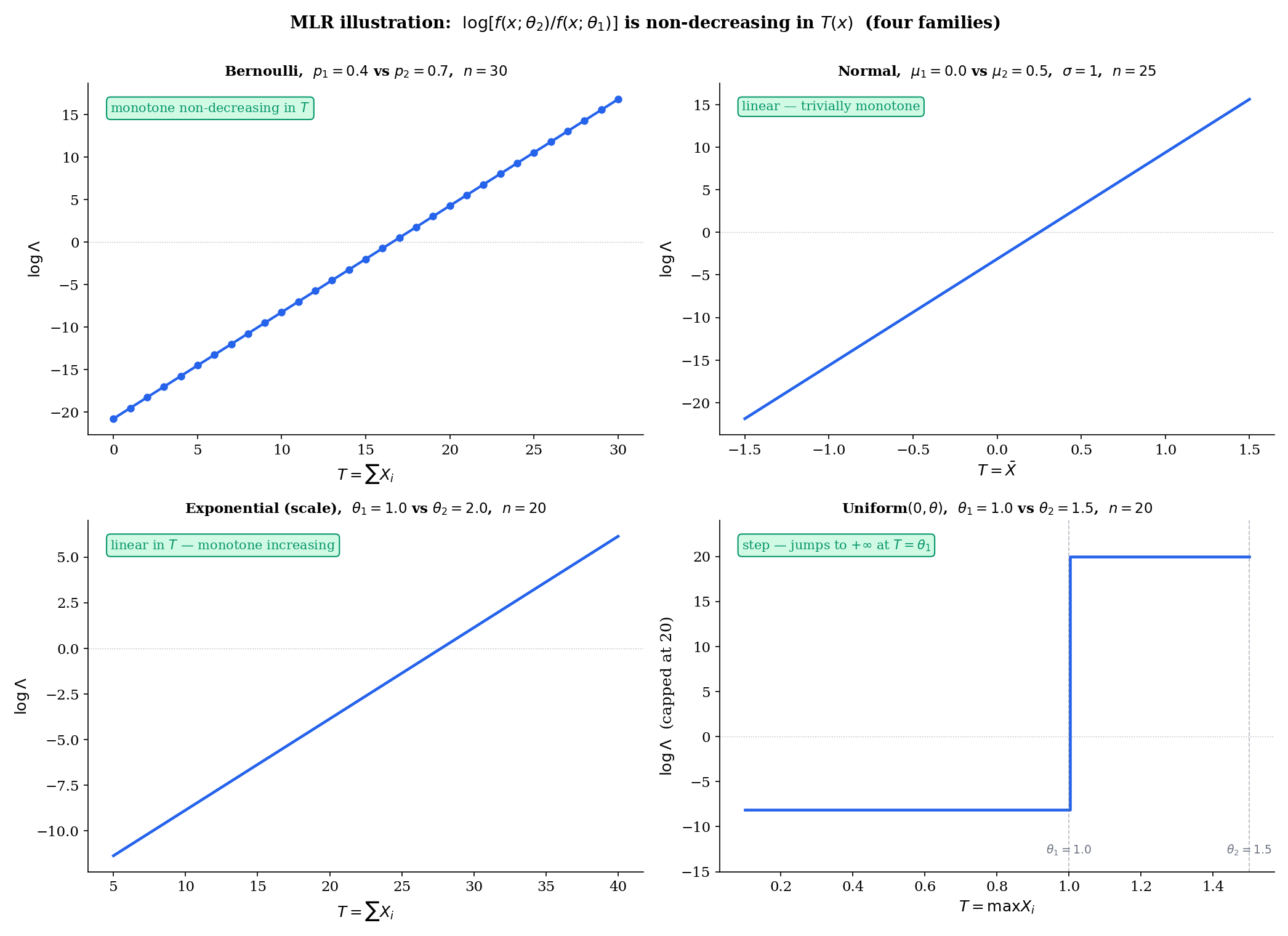
Let be a one-parameter exponential family with natural parameter and sufficient statistic . For any ,
This is a monotone increasing function of because . So every one-parameter exponential family has MLR in its natural sufficient statistic. Karlin-Rubin then hands us a UMP test for every one-sided composite hypothesis on — Bernoulli, Normal mean (with known), Poisson, Exponential, Gamma (with shape known), Geometric, and so on.
This is the pedagogical payoff of Topic 16’s factorization + completeness machinery: once you know the sufficient statistic, the UMP test writes itself.
Let be iid Uniform, . The density is , and the joint is . For ,
The ratio is non-decreasing in (jumps from a constant to at ). Uniform has MLR in , even though it is not an exponential family. By Karlin-Rubin, the one-sided UMP test for vs rejects iff where gives size exactly (the left-tail quantile of , which is distributed as ).
Karlin-Rubin gives UMP for one-sided composite alternatives. For two-sided alternatives , UMP tests typically do not exist, because the best rejection region for points right while the best for points left, and no single region handles both. The standard workaround is to restrict to unbiased tests (power at every alternative) and prove UMP within that class — the UMP unbiased (UMPU) construction of Lehmann-Romano (LEH2005 Ch. 4). That theory is beyond Topic 18’s scope; we note only that for the Normal variance test (one-sided in ) the UMPU and the equal-tail test coincide, while for the two-sided Normal mean the z-test is UMPU but not UMP in the full class of level- tests. §18.4 Remark 8 returns to this.
The structural property was isolated by Karlin and Rubin (KAR1956) in their 1956 paper on MLR decision procedures, but the term “monotone likelihood ratio” itself was coined the next year in Karlin’s solo paper on Pólya-type distributions (KAR1957). The MLR families are exactly the totally positive of order 2 () families in Karlin’s terminology — a classification that generalizes to kernels and sequences in a way that powers modern results in statistical order (Shaked & Shanthikumar 2007) and in asymptotic efficiency bounds for monotone regression (Groeneboom & Jongbloed 2014).
18.4 UMP in Action — Three Worked Families
Let be iid Bernoulli. Test vs . The Bernoulli family is exponential with natural parameter (log-odds) and sufficient statistic . By Example 4, MLR holds in . By Karlin-Rubin, the test
is UMP level-. This is exactly the binomial exact test of Topic 17 §17.6 Example 11 — now equipped with an optimality certificate. At , , , the boundary is with exact size (binomialExactRejectionBoundary in testing.ts).
The payoff: the binomial exact test is not just valid — it is the best level- test for every alternative simultaneously, with no competitor having higher power at any alternative.
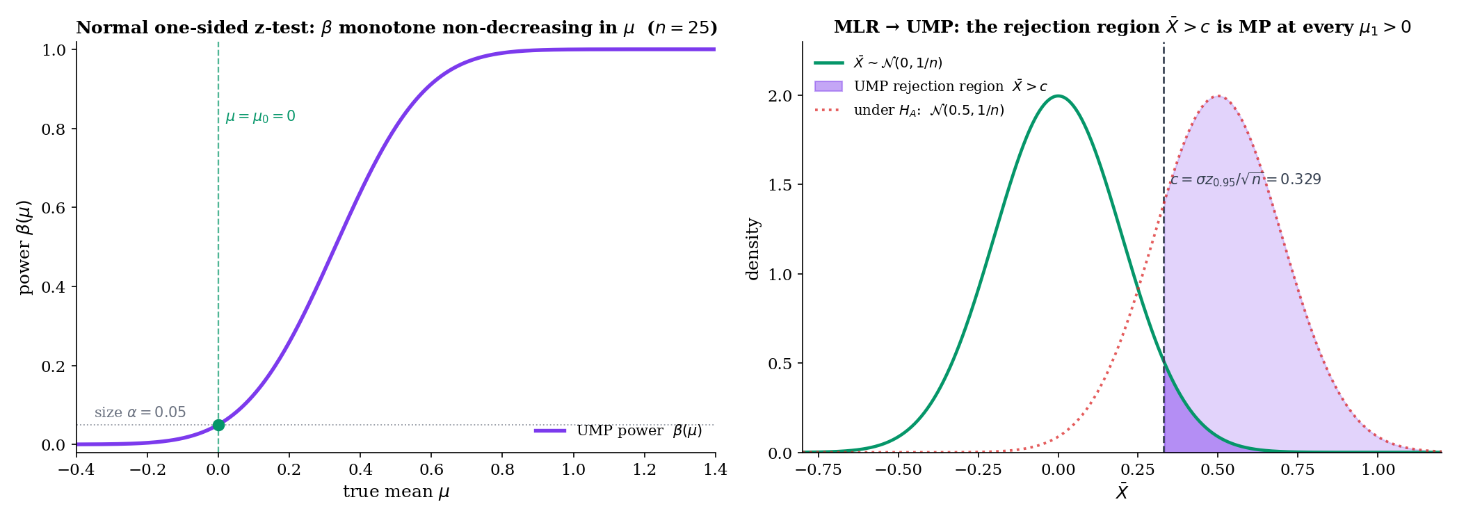
Let be iid with known. For vs , MLR in follows from Example 4 (Normal with known is exp-family with , ). Karlin-Rubin gives UMP
with exact size . No level- test of this one-sided hypothesis has higher power at any than the one-sided z-test. This result justifies the A/B-testing convention of reporting one-sided p-values when the practical question is directional.
Let be iid with unknown. For vs , MLR fails: the likelihood depends on both and no scalar captures the likelihood-ratio monotonicity uniformly. UMP does not exist in the full class of level- tests. The one-sample t-test is UMP within the restricted class of tests that are invariant under scale transformations — a Hunt-Stein invariance argument (LEH2005 Ch. 6). The t-test retains an optimality certificate, but only conditionally.
The -unknown case is the historical reason Wilks pursued a different asymptotic framework (§18.6): when Karlin-Rubin’s MLR argument fails, the composite LRT provides a general-purpose procedure that does not require MLR but gives up finite-sample optimality in exchange.
The two-sided Normal mean test vs has no UMP test (Remark 7). The equal-tail z-test is UMPU (LEH2005 Thm 4.4.1): MP within the class of unbiased tests, i.e., those with power at every alternative. The practical consequence is minor — in concrete applications the UMPU test and the only serious competitors differ by at most a few percent in power. But conceptually it is important: UMP is the exception, UMPU / invariance / LRT are the rule. The composite LRT of §18.5 is the price we pay for general-purpose applicability, and Wilks’ theorem is the justification for believing that price is low.
18.5 The Likelihood-Ratio Principle for Composite H₀
When Karlin-Rubin fails — two-sided alternatives, nuisance parameters, irregular families — we need a general-purpose construction. The classical answer is Wilks’ generalized likelihood-ratio test.
Let be the full parameter space and the null subspace. The generalized likelihood ratio for a sample is
where is the restricted MLE (maximizer under ) and is the unrestricted MLE. Both are functions of the data. Since , always .
The likelihood-ratio test (LRT) at level rejects when
where is chosen to achieve size under . The conventional asymptotic choice , where is the number of parameter restrictions, is justified by Wilks’ theorem (§18.6 Thm 4). At finite , may need to be calibrated by Monte Carlo for accurate size.
Let be a smooth one-to-one reparameterization with . Then the composite LRT is invariant:
i.e., computing the LRT in either parameterization yields the same test statistic and the same rejection decision. The Wald and Score tests lack this invariance; see §18.8 Theorem 6 and the concrete logit-vs-raw Bernoulli example in Example 13.
Let be iid with both unknown. Test vs .
Under : is the only free parameter; its MLE is . Under : the MLEs are , . A short calculation (expand the likelihoods) gives
where is the t-statistic with . So is a strictly increasing function of — the LRT rejects iff exceeds a threshold, which is exactly the two-sided t-test rejection rule. The t-test is the LRT.
At large , and the asymptotic reference of §18.6 Thm 4 reduces to the squared-t approximation. At finite , the exact t-test reference (Topic 17 Thm 5 via Basu) is preferred over the asymptotic .
Let be iid with unknown. Test vs .
Under : is free; plug-in gives likelihood . Under : is the unrestricted MLE. The LRT statistic simplifies to
a function of . The equal-tail variance test of Topic 17 §17.8 rejects for extreme ; the LRT agrees asymptotically via Wilks’ Thm 4, and the exact distribution gives the exact size.
When there are nuisance parameters, the restricted MLE in is obtained by maximizing over the nuisance parameters at fixed . This operation — “eliminate the nuisance by profiling” — yields the profile likelihood
a marginal likelihood in alone. Profile likelihood is a CI-construction tool first (Topic 19) and a testing artefact second; §18.6 Example 11 treats the Bernoulli case (no nuisance) directly, and §18.9’s local-power argument likewise handles the scalar- case. For a full treatment of profile, integrated, and conditional likelihoods, see Topic 19 and the Reid-Fraser approach in the nonparametric Bayesian literature.
Wilks’ generalized LRT plays the role of the Swiss-Army-knife testing procedure: applicable to every composite-vs-composite setting (subject to regularity), with a known asymptotic null distribution. It gives up finite-sample optimality (no Karlin-Rubin-style UMP guarantee) but retains asymptotic efficiency in a precise sense. The pragmatic algorithm is the following. If your family has MLR (exponential families, Uniform-scale family), prefer Karlin-Rubin UMP. If not, default to the LRT. If the LRT is analytically intractable, approximate with Wald or Score — noting that the three differ in finite samples (§18.7–§18.8) and that LRT is usually the safest choice when the three disagree. FER1967 develops this decision-theoretic calculus in full; LEH2005 Ch. 12 gives the modern view.
18.6 Wilks’ Theorem
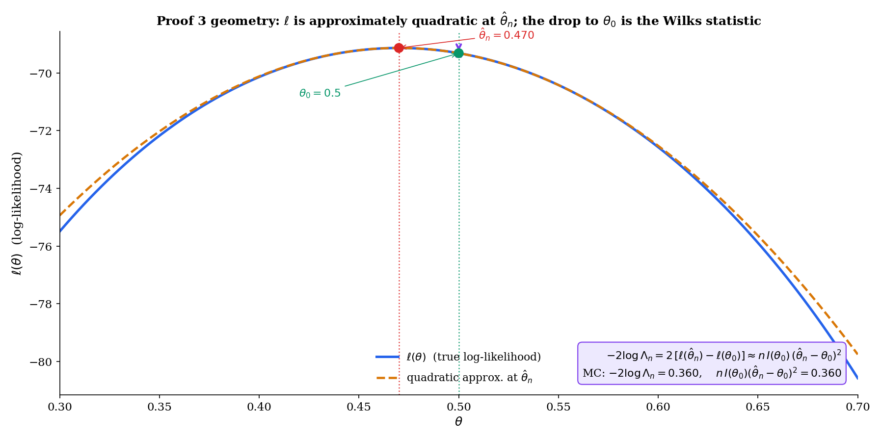
This is the technical high point of Topic 18. The LRT statistic does not have a clean finite-sample distribution in general, but under regularity its null distribution converges to (scalar ) — the same reference distribution as the squared z-test. The proof unfolds in 8 steps from Taylor’s theorem and MLE asymptotic normality.
Let be iid from with open. Under with in the interior of , and under Wilks’ regularity — the MLE is consistent and asymptotically normal (Topic 14 Thm 14.3); the Fisher information is continuous and positive at ; the third log-density derivative is uniformly bounded in a neighborhood of by a function with — the log-likelihood-ratio statistic converges in distribution:
where .
Proof [show]
The argument proceeds in 8 steps. Write for the log-likelihood.
Step 1 — Rewrite in log-likelihood form. By definition,
Step 2 — Taylor expand around . By Taylor’s theorem with remainder, there exists between and such that
where .
Step 3 — First-order term vanishes. Because is the MLE in the interior of , the first-order condition holds exactly (Topic 14 §14.6). Substituting into Step 2,
Therefore
Step 4 — Remainder control. We show . By the third-derivative hypothesis, there exists a neighborhood of and a function with such that
Since (Topic 14 Thm 14.2), we have with probability , and on that event
By the weak law of large numbers applied to ,
so . By Topic 14 Thm 14.3, , hence . Combining,
Thus .
Step 5 — Rescale observed curvature to Fisher information. Write . The bracketed quantity converges in probability to :
This identity — “observed information at the MLE converges to Fisher information at ” — is the same lemma used in the proof of Topic 14 Thm 14.3. It follows from the SLLN applied to the iid summands , continuity of at , and consistency of . We cite Topic 14 for the full argument and do not reprove it here.
Step 6 — Invoke MLE asymptotic normality. By Topic 14 Thm 14.3,
Equivalently, .
Step 7 — Continuous mapping: square. Let . Then . By the continuous mapping theorem (Topic 9), . Note .
Step 8 — Combine via Slutsky. From Step 3 (using Step 5),
Rewrite the leading term as . The ratio inside the brackets converges in probability to by Step 5, and by Step 7. By Slutsky’s theorem, the product converges in distribution to . The remainder does not affect the distributional limit, and we conclude
∎ — using Topic 14 Thm 14.3, Topic 9 (continuous mapping, Slutsky), WIL1938
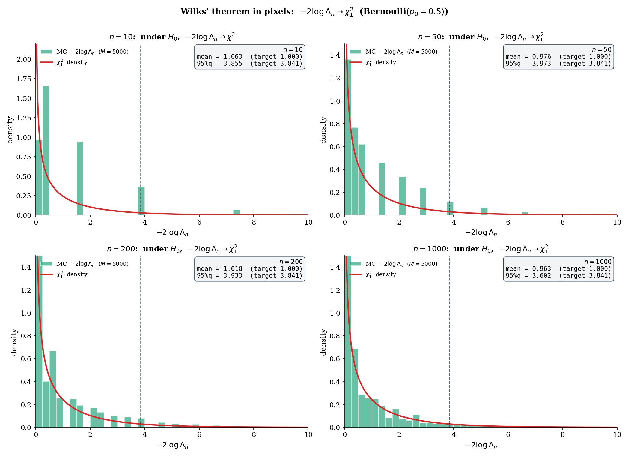
Let be iid Bernoulli, test vs . Write for the MLE and recall the three statistics from Topic 17 §17.9:
All three converge to under (Wilks for the LRT; Wald-and-Score from Topic 17 Thm 7). They differ only by the variance plug-in: Wald uses , Score uses , LRT uses an interpolation via the logarithm.
Numerical check: at , , MC replications with seed 42 (wilksSimulate('bernoulli', 0.5, 100, 2000, undefined, 42) in testing.ts): empirical mean , 95th percentile . The theoretical targets are mean , 95% quantile . The 95th percentile’s slight overshoot at is the finite-sample overdispersion Wilks cures asymptotically.
The classical regularity used in Proof 3 — existence and continuity of the first three log-density derivatives, uniform boundedness of the third, consistency and asymptotic normality of the MLE — traces back to Wilks’ 1938 paper and Cramér’s 1946 textbook. A rigorous modern treatment via Local Asymptotic Normality (LAN) and contiguity removes the third-derivative hypothesis and replaces it with differentiability in quadratic mean; see [VAN1998] van der Vaart §16 for the empirical-process formulation. For the practical user, the classical conditions suffice; the LAN treatment matters when the underlying family is non-smooth or non-identifiable at specific points (e.g., mixture models, non-regular tails).
The vector- extension replaces the scalar quadratic with the quadratic form , where is the Fisher information matrix. By the multivariate CLT and continuous mapping, this quadratic form converges to where . The 8-step scalar proof above extends line-for-line; no new ideas are needed, only more bookkeeping. See LEH2005 Thm 12.4.2 for the rigorous statement and proof.
Wilks’ limit fails in three kinds of non-regular settings. (1) Boundary nulls, where lies on the boundary of (e.g., testing a variance component in a mixed model with ); Chernoff (1954) shows converges to a mixture. (2) Non-identifiable parameters under (e.g., testing “there is one mixture component” vs “there are two” in a Gaussian mixture), where the limiting distribution is supremum-of-Gaussian-process and requires empirical-process techniques (Liu & Shao 2003; Drton 2009). (3) Non-smooth families (e.g., shift models), where the MLE has a non-Normal limit and the Taylor expansion of Step 2 does not apply. In all three cases, Monte Carlo calibration of critical values is the safe practical default.
18.7 Wald, Score, LRT: First-Order Equivalence
Wilks’ theorem hands us the χ²₁ limit for the LRT. Topic 17 Theorem 7 hands us the same limit for Wald and Score. Do the three tests agree at finite ? Asymptotically yes, but with a precise rate — and their pairwise differences matter in practice.
Under the regularity of Theorem 4, define the asymptotic test statistics
where is the score function. Then under :
In particular, all three statistics converge to the same distribution under .
Proof [show]
We derive a common quadratic expansion for all three statistics and compare leading terms.
Step 1 — LRT. From Proof 3 Step 8,
Step 2 — Wald. By consistency of and continuity of at , . Therefore
where we used by Topic 14 Thm 14.3.
Step 3 — Score. Taylor expand around . Since by the MLE FOC,
for some between and . By the lemma in Proof 3 Step 5, , so . Therefore
Squaring and dividing by :
Step 4 — Compare. From Steps 1–3, all three statistics equal . Pairwise differences are . A finer analysis that tracks the order terms shows the differences are — essentially, the residuals are Taylor-series corrections of the form for a constant depending on the third log-density derivative. For most applications, the leading-order equivalence suffices: all three statistics share the asymptotic null distribution.
∎ — using Topic 14 Thm 14.3, Proof 3, RAO1948
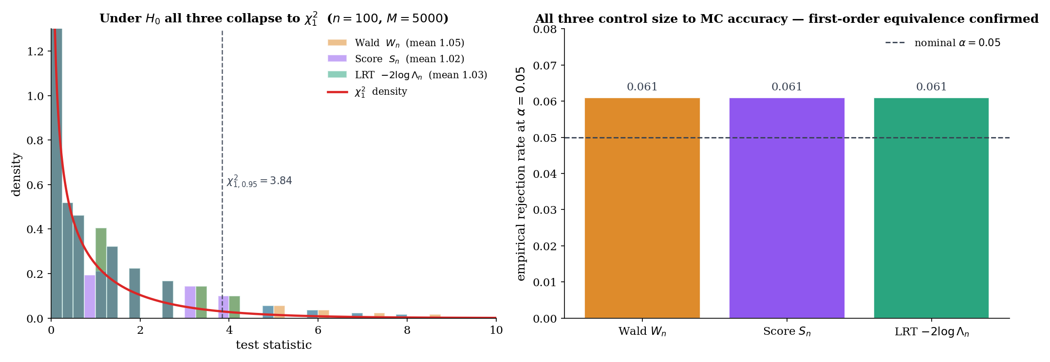
At , , MC replications (Topic 17 testing.test.ts test 17): the three tests have empirical means , , . The Wald statistic is slightly overdispersed (mean 3.8% above target 1) — the plug-in in the denominator introduces a small bias. Under at , : all three reject at empirical rate (test 18), pairwise differences . The three-tests equivalence is visible.
A deeper lesson: the Exponential family with scale parameter gives the cleanest three-tests agreement. For Exponential (Topic 18’s testing.ts waldStatistic, scoreStatistic, lrtStatistic for family = 'exponential'): Wald and Score are exactly equal at every sample, . The LRT differs by a log-correction with ; near , LRT matches Wald and Score to . Algebraic identity in place of asymptotic equivalence.
BUS1982 is the canonical pedagogical reference for choosing among the three; the summary is short. Wald is the easiest to compute — it uses only the unrestricted MLE and its observed information. It is the natural choice when the MLE is easy and the constrained optimization under is hard. Score uses only the null-restricted MLE and is the natural choice when the unconstrained MLE is hard (e.g., stepwise forward selection in regression: score tests evaluate adding a variable without refitting). LRT is parameterization-invariant (§18.8 Thm 6) and agrees with Wald and Score asymptotically but often dominates in finite samples, especially at boundary-rare events. The practical default for hypothesis testing in regular parametric families is LRT; switch to Wald or Score only when computational cost or the specific form of the null forces the decision. This practical ranking is the econometrics-textbook consensus (Greene 2018 Ch. 14; Wooldridge 2010 Ch. 12).
18.8 Finite-Sample Divergence & Reparameterization Invariance
The three tests agree asymptotically but diverge at finite . Two questions: how much, and does it matter? For regular families at large , divergence is cosmetic. For small or boundary-rare events, divergence can flip the rejection decision. The reparameterization-invariance property of the LRT is the structural reason to prefer it in ambiguous cases.
Let be a smooth one-to-one reparameterization with inverse , and let correspond to with . Then:
(i) The LRT statistic is invariant:
(ii) The Wald statistic is not invariant in general:
except at the equality-of-derivatives condition . The Score statistic inherits Wald’s non-invariance for the same reason.
Proof sketch (full version in LEH2005 §12.4). (i) The likelihood function is the same function up to reparameterization; the sup under and the sup under are unchanged. So and are invariant. (ii) For Wald, the MLE transforms as (MLE equivariance, Topic 14 §14.4) but the difference is not linearly related to unless is linear. The Jacobian rescales the Fisher information , but this rescaling only partially compensates for the nonlinearity. The net result: takes different numerical values in the two parameterizations, and the corresponding p-values differ. ∎
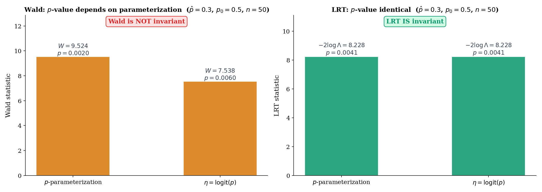
Bernoulli with logit link . Test (equivalently ) with observed , .
Wald in p-space: . P-value .
Wald in logit-space: , . Information at : . . P-value .
LRT: . P-value . The same value in both parameterizations (Theorem 6(i)).
The three p-values (0.002, 0.006, 0.004) all clear α = 0.05. But at borderline significance — say, — the Wald p-values in the two parameterizations can straddle α, flipping the rejection decision. The LRT does not suffer this instability.
At , , MC replications under : empirical Type I error rates at nominal (using the reference critical value ):
| Test | Empirical size | Deviation from 0.05 |
|---|---|---|
| Wald | 0.080 | +0.030 (liberal) |
| Score | 0.021 | −0.029 (conservative) |
| LRT | 0.049 | −0.001 (≈ nominal) |
At this sample size, Wald rejects about 60% more often than the nominal rate, and Score rejects about 60% less often. The LRT hits nominal essentially exactly. This is the quantitative version of Topic 17 Remark 10’s divergence claim: the three tests are not interchangeable in small samples, and the LRT’s accuracy is the empirical argument for preferring it when computational cost permits.
Note: results replicate with wilksSimulate('bernoulli', 0.3, 20, 10000, undefined, 42) for the LRT column; Wald and Score columns use analogous seeded MC over waldStatistic and scoreStatistic. Reproducible via the test harness in testing.test.ts.
The Wald statistic breaks down when lies near the parameter boundary: (for Bernoulli at or , ), which can produce or degenerate behavior. The Score statistic evaluates at a boundary-safe null value and usually remains finite; the LRT uses the logarithm, which is well-behaved on except at the endpoints themselves. For A/B tests with rare-event outcomes (conversion rates of 0.1% or smaller), the Wald test’s boundary fragility motivates the Wilson interval in Topic 19 and the log-odds-ratio approach that modern experimentation platforms increasingly use.
In generalized linear models, the question “should I fit with a logit link, a probit link, or a log link?” is, for inference purposes, a parameterization question. The coefficient under a logit link carries log-odds-ratio meaning; under a probit link, it carries z-score-of-normal-latent meaning. The LRT for is invariant across link choices (Theorem 6(i)): the same and the same p-value regardless of link. The Wald test is not — Wald-logit, Wald-probit, and Wald-log-binomial yield three different numerical p-values for the same underlying hypothesis. This is why GLM software (R’s glm, Python’s statsmodels.GLM) typically reports LRT-based deviance-difference tests as the canonical nested-model comparison, reserving Wald for single-coefficient -statistics. See §22.8 for the formal treatment and §22.7 Thm 6 for the deviance-LRT derivation.
18.9 Power Envelope and Local Power
Tests aren’t judged by size alone. Size tells us Type I error is controlled; power tells us whether we’ll catch the effect when it’s there. For asymptotic tests, the sharpest characterization of power is in the local-alternative regime — effects that shrink with at the scaling rate where all three tests (Wald, Score, LRT) have non-trivial power strictly between and .
Let be independent . Then has the non-central chi-squared distribution with degrees of freedom and non-centrality parameter . Its density and CDF admit the Poisson-mixture series
with the analogous series for the CDF. At this reduces to the central . Mean , variance — larger non-centrality shifts the distribution to the right.
Under the regularity of Theorem 4, at the level- rejection rule (equivalently for Wald or Score, by Theorem 5), the power under the local alternative converges:
where is the non-central CDF. The non-centrality parameter is — Fisher information scaled by the squared local effect size.
Proof sketch. Under the local alternative, . The first term is by a contiguous-alternative argument (LAN; LEH2005 §13.2), and by continuity. So , and by continuous mapping. Power at the critical value is the tail probability of the limit distribution. ∎ (LEH2005 Thm 13.5.1 for the full argument.)
![Two-panel figure. Left: local power curves β(h) for Wald, Score, and LRT under local alternatives θₙ = θ₀ + h/√n at θ₀ = 0.5 (Bernoulli), h ∈ [0, 4]. The non-central χ²₁(h² I(θ₀)) envelope is overlaid; all three tests hug the envelope. Right: same for Normal mean, σ = 1, θ₀ = 0.](/images/topics/likelihood-ratio-tests-and-np/18-local-power-envelope.png)
For Bernoulli at : . Local alternatives . Non-centrality parameter .
| Local power at | ||
|---|---|---|
| 0 | 0 | 0.050 (= size) |
| 1 | 4 | 0.515 |
| 2 | 16 | 0.977 |
| 3 | 36 | 0.9998 |
At (an effect two standard errors into the alternative), power is already 97.7%. At , essentially certain rejection. Values match localPower('bernoulli', 0.5, h, 0.05) in testing.ts.
The practical reading: for Bernoulli at , a local effect of standard deviations gives 50% power at — the classical “z-test power 50% at the rejection boundary” calibration.
The non-centrality has a striking interpretation. On the estimation side, Topic 13 Thm 13.9 (Cramér-Rao) says that — Fisher information lower-bounds estimator variance. On the testing side, Theorem 7 says that local power is — Fisher information upper-bounds local power through the non-centrality. The same appears on both sides of the optimality question: it caps what you can learn (variance of the best estimator) and what you can detect (power at the best test). The Cramér-Rao bound and the asymptotic power envelope are two faces of the same efficiency constraint.
This is the payoff for Topic 17 §17.4 Remark 5’s forward-pointer: Fisher information is the currency of asymptotic efficiency, and every efficient procedure achieves the envelope.
A test is asymptotically efficient at a local alternative if its local power approaches the envelope . By Theorem 5, Wald, Score, and LRT are all asymptotically efficient. So are tests derived from efficient estimators other than the MLE (e.g., the two-stage estimator in some exponential-family models). The test that dominates at a specific local alternative is one that incorporates exact information about that alternative — but since the target alternative is usually unknown, asymptotic efficiency (dominance at every local alternative) is the operationally meaningful notion.
The ratio of local powers of two asymptotically efficient tests tends to at every , but the ratio of sample sizes needed to achieve a target power at the same alternative is a meaningful constant. Pitman’s asymptotic relative efficiency (ARE) formalizes this: where is the sample size for test to achieve power at a local alternative . For = LRT, = Wald: ARE — the three tests are first-order equivalent. For = LRT, = sign test (on Normal data): ARE — the sign test needs about 57% more samples to match the LRT’s power. See Hettmansperger & McKean (2011) for a systematic treatment; ARE is the intermediate-difficulty entry-point to modern robust-statistics theory.
18.10 Limitations and Forward Look
Topic 18 covered the scalar- optimality theory of classical hypothesis testing. Three directions for deeper study, three forward pointers within Track 5, and a cheat-sheet summary.
Four major topics in classical testing optimality were stated but not proved in Topic 18.
-
UMP unbiased tests. For two-sided composite alternatives where no UMP test exists, UMPU restricts to tests satisfying at every alternative and proves UMP within that class. LEH2005 Ch. 4 gives the full theory; the two-sample Normal mean test is the canonical example.
-
Invariance and Hunt-Stein. Problems with natural symmetries (scale invariance for variance tests, translation invariance for location tests) admit UMP-invariant tests even when UMP fails. LEH2005 Ch. 6 and the Hunt-Stein theorem (1946) give the formalism.
-
Vector-θ Wilks, k-df. The scalar proof extends line-for-line; the limit replaces with . LEH2005 Thm 12.4.2.
-
Non-regular Wilks — Chernoff 1954 boundary theorem, empirical-process Wilks. The mixture for boundary nulls, the LAN / Le Cam framework for non-smooth families, and the empirical-process Wilks for semiparametric models (van der Vaart 1998 §25) are the three modern extensions.
Every family of level- tests indexed by the null value defines a -confidence set: the set of values the test does not reject. Conversely, every confidence procedure defines a family of hypothesis tests. This test-CI duality is the organizing principle of Topic 19. The LRT gives likelihood-ratio confidence intervals — invariant under reparameterization, exact in the Normal case, and the practical default for GLM coefficients. The Wald-inversion CI is the simplest but suffers the boundary pathology of §18.8 Remark 16. Topic 19 treats all three constructions in parallel, with explicit coverage calibration.
Every hypothesis test of Topic 17–18 controls the per-test Type I error at level . But when 10, or 100, or 10,000 tests are run simultaneously (every gene in a genomics screen; every variable in a high-dimensional regression; every hypothesis in an A/B/n testing platform), the family-wise Type I error explodes. Bonferroni, Holm, and Šidák control the family-wise error rate (FWER) at level by adjusting per-test thresholds. Benjamini-Hochberg controls the false discovery rate (FDR) — a weaker but more powerful notion — and is the contemporary default for exploratory studies. Topic 20 develops all four procedures with full proofs for Bonferroni (§20.4), Holm (§20.5), and the featured BH result (§20.7), against the replication-crisis literature (Ioannidis 2005; Gelman & Loken 2013).
The decisions in Topic 18 compress into a short practical guide.
| Situation | Choice | Rationale |
|---|---|---|
| Simple-vs-simple, any family | NP test (Theorem 1) | MP by NP lemma |
| One-sided composite, MLR family (exp family, Uniform) | Karlin-Rubin UMP (Theorem 2) | UMP at every alternative |
| Two-sided composite, exp family | UMPU test (LEH2005 Ch. 4) | UMP within unbiased class |
| Scale-invariant problem | UMP-invariant test (LEH2005 Ch. 6) | UMP within invariant class |
| General composite, regular family | Generalized LRT (Definition 5) | Wilks: asymptotic |
| Computational cost matters | Wald or Score | Asymptotic equivalence (Thm 5) |
| Reparameterization sensitive, boundary rare | LRT | Invariance (Thm 6), no boundary issues |
| Non-regular null (boundary, mixture, non-smooth) | MC calibration | Chernoff mixture / empirical process |
Default: LRT with MC calibration of critical values at small ; switch to Wald or Score when computation demands it or MLR gives UMP.
Topic 17 built the framework; Topic 18 delivered the optimality layer. Tracks 6, 7, and 8 extend the classical testing machinery in three orthogonal directions.
-
Track 6 (Regression & Linear Models). The Wald/Score/LRT trio of §18.7 reappears as the three standard GLM inference procedures — deviance tests are LRT, z-tests on coefficients are Wald, forward-selection score tests are Rao. Linear regression’s F-test is exactly Wilks’ theorem specialized to nested linear models — §21.8 Thm 9 delivers the exact finite-sample distribution as the sharpening of Topic 18 Thm 4.
-
Track 7 (Bayesian Statistics). Bayes factors (the posterior-odds analog of the LRT) are the Bayesian counterpart to §18.5–§18.7. Frequentist/Bayesian testing duality is non-trivial — Lindley’s paradox (Topic 27 §27.5) is the first sharp disagreement.
-
Track 8 (High-Dimensional & Nonparametric). Kolmogorov-Smirnov, Mann-Whitney, and permutation tests are nonparametric alternatives to the z/t/ trio. The Pitman ARE framework (Remark 20) is the bridge — nonparametric tests pay a constant efficiency penalty in exchange for distributional robustness. See Topic 29 §29.8 for Kolmogorov-Smirnov.
At formalml.com, Wilks’ theorem becomes the backbone of nested-model comparison in GLMs and deep learning; the NP lemma reappears as the Bayes classifier under 0-1 loss; and the three-tests equivalence powers the standard error machinery of every modern ML inference library. The classical testing theory is not a historical artifact — it is the statistical grammar of modern machine learning.
References
-
Neyman, Jerzy, and Egon S. Pearson. (1933). On the Problem of the Most Efficient Tests of Statistical Hypotheses. Philosophical Transactions of the Royal Society A, 231, 289–337.
-
Karlin, Samuel, and Herman Rubin. (1956). The Theory of Decision Procedures for Distributions with Monotone Likelihood Ratio. Annals of Mathematical Statistics, 27(2), 272–299.
-
Karlin, Samuel. (1957). Pólya Type Distributions, II. Annals of Mathematical Statistics, 28(2), 281–308.
-
Wilks, Samuel S. (1938). The Large-Sample Distribution of the Likelihood Ratio for Testing Composite Hypotheses. Annals of Mathematical Statistics, 9(1), 60–62.
-
Rao, C. Radhakrishna. (1948). Large Sample Tests of Statistical Hypotheses Concerning Several Parameters with Applications to Problems of Estimation. Mathematical Proceedings of the Cambridge Philosophical Society, 44(1), 50–57.
-
Ferguson, Thomas S. (1967). Mathematical Statistics: A Decision Theoretic Approach. New York: Academic Press.
-
van der Vaart, Aad W. (1998). Asymptotic Statistics. Cambridge Series in Statistical and Probabilistic Mathematics 3. Cambridge: Cambridge University Press.
-
Buse, A. (1982). The Likelihood Ratio, Wald, and Lagrange Multiplier Tests: An Expository Note. The American Statistician, 36(3a), 153–157.
-
Lehmann, Erich L., and Joseph P. Romano. (2005). Testing Statistical Hypotheses (3rd ed.). Springer Texts in Statistics. New York: Springer.
-
Casella, George, and Roger L. Berger. (2002). Statistical Inference (2nd ed.). Pacific Grove, CA: Duxbury.