Kernel Density Estimation
The kernel density estimator, the AMISE bias–variance decomposition, the optimal bandwidth h* of order n^(−1/5), Epanechnikov's optimal-kernel theorem, Parzen's pointwise asymptotic normality, and data-driven bandwidth selectors (Silverman, Scott, UCV, Sheather–Jones). Track 8, topic 2 of 4.
30.1 Motivation: from ECDF to density
Topic 29 built its entire nonparametric toolkit on the empirical CDF — a step function that converges uniformly to the true CDF . But is not differentiable, so the density is unreachable by naïve differentiation. Kernel density estimation is the answer to the obvious question: what happens when we differentiate using a smooth weighting function instead of a Dirac delta?
The idea is simple enough to state in a sentence. Replace each sample point with a small bump of area centered at ; add the bumps up. The sum is a bona fide density (nonnegative, integrates to 1) that looks like as grows, with a smoothness controlled by the bump width. Histograms are the roughest version — rectangular bumps of constant width, anchored to arbitrary bin edges. KDE replaces those rectangles with a smooth, symmetric, nonnegative kernel and drops the bin-edge arbitrariness entirely.
Figure 1 takes a single Normal sample of size and plots three histograms (bin widths ) alongside three Gaussian-kernel KDEs (bandwidths ). At small or small , both estimators are spiky and variance-dominated; at large or large , both over-smooth and bias-dominate. The KDEs remove one obvious source of arbitrariness — bin edges — but the bandwidth problem remains, just in a smoother form.
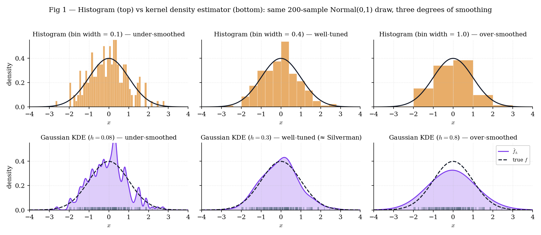
Figure 1. Histograms (top) and KDEs (bottom) on the same Normal sample. The bin-width / bandwidth trade-off between spikiness and over-smoothing is visible in both rows; KDE removes the bin-edge arbitrariness but keeps the smoothing-parameter choice.
Histograms have two genuine advantages KDEs lack: they are exactly piecewise-constant (so integrals over bin intervals are trivial) and they are visually honest about the underlying empirical counts. KDEs are smoother and easier to differentiate further (for mode-finding or density-gradient methods), but the smoothness is imposed, not inherent. A reader who wants to know “how many data points fell in ?” should look at a histogram; a reader who wants a differentiable density estimate should look at a KDE.
Topic 7 built density families (Normal, Gamma, Beta) and fit parametric from data. That program is efficient when the family is right and biased when it’s wrong. KDE drops the family assumption and estimates directly from the sample — a distribution-free procedure in the sense of Topic 29 §29.1 Rem 1. The price is a slower convergence rate: we’ll see in §30.6 that AMISE decays at , slower than the parametric , and that this is the price of distribution-freeness.
30.2 The kernel density estimator
With the motivation out of the way, we can write down the estimator formally and check that it is a density. Three definitions (kernel, scaled kernel, KDE) and one stated theorem (KDE is a valid density) — enough to set up everything that follows.
A kernel is a function satisfying
Nonnegativity and unit mass make a density on ; symmetry makes it a density centered at . We additionally require finite variance and finite roughness , both used throughout §30.4–§30.6.
For bandwidth , the scaled kernel is
The scaling preserves the density property — for any — and turns into a width parameter: small makes tall and narrow (close to a Dirac delta); large makes it short and wide.
Given an iid sample from an unknown density , the kernel density estimator with kernel and bandwidth is
Both forms are in active use. The first makes it visually obvious that is an average of kernel-shaped bumps centered at the data. The second groups the bandwidth normalization into a single factor, which will be convenient when we compute bias and variance in §30.4.
Under the definitions above, is a bona-fide probability density:
Stated; the proof is elementary. Nonnegativity is immediate from . Integration reduces to by the scaled-kernel normalization.
Take observations , and Gaussian kernel . At bandwidth :
where we used . The KDE at the midpoint receives equal contribution from both observations and is therefore twice . This is the T30.8 test pin — a two-point sanity check on the kdeEvaluate implementation.
Writing for the empirical distribution (a probability measure that places mass at each sample point), we have . KDE is the convolution of a smooth kernel with the empirical distribution — equivalently, it is the empirical density against a smoothed observation model. This formulation is convenient in formalml where the convolution structure generalizes to multivariate bandwidths and non-iid samples.
Symmetry makes the first-moment condition automatic, which simplifies the bias calculation in §30.4 (the Taylor term drops out). Nonnegativity guarantees , so the estimator is always a valid density. A fourth-order or higher-order kernel with can achieve faster bias rates (down to ) but requires to take negative values, and then may be negative in places — a practical complication we’ll mention in §30.6 Rem 13 and defer to Serfling 1980 §1.11.
30.3 Kernels: families and properties
Five kernels are standard — Gaussian, Epanechnikov, biweight (quartic), triangular, and uniform — and every modern implementation supports all five. The constants that govern AMISE ( and ) are closed-form for each, and their efficiency relative to Epanechnikov sits between 0.93 and 1.00 across the whole family. Kernel choice, in practice, matters much less than bandwidth choice.
The five standard symmetric kernels, with their second moments and roughness:
| Kernel | Support | Efficiency | |||
|---|---|---|---|---|---|
| Gaussian | |||||
| Epanechnikov | $\frac34(1 - u^2)\mathbf1{ | u | \le 1}$ | ||
| Biweight | $\frac1516(1 - u^2)^2\mathbf1{ | u | \le 1}$ | ||
| Triangular | $(1 - | u | )\mathbf1{ | u | \le 1}$ |
| Uniform | $\frac12\mathbf1{ | u | \le 1}$ |
Stated. All values are elementary integrals; Example 3 verifies Epanechnikov explicitly, and the kernelProperties export in nonparametric.ts §8 encodes all five (T30.5–T30.6).
For :
The values and are load-bearing for Theorem 5’s Epanechnikov optimality proof in §30.6.
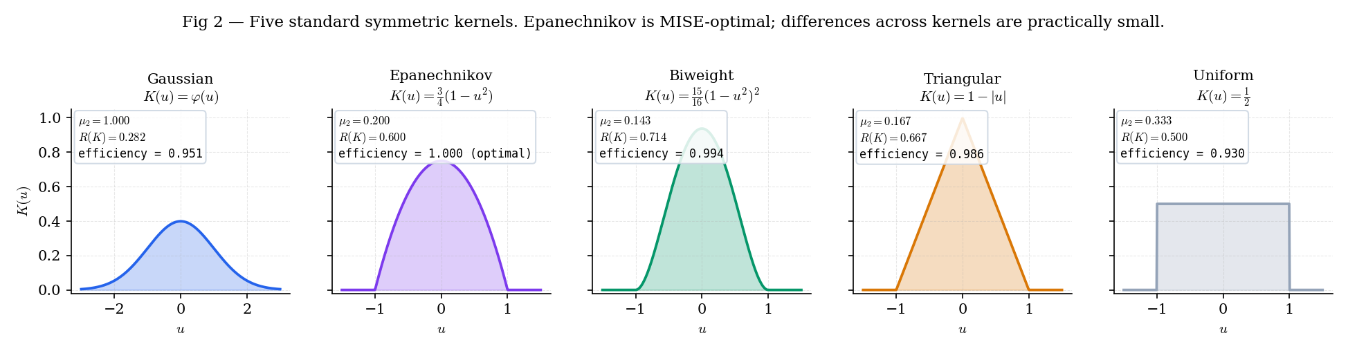
Figure 2. The five standard kernels on a common axis. Gaussian extends into the tails; the other four have compact support on . Efficiency — the figure of merit from §30.6 Theorem 5 — ranges from (uniform) to (Epanechnikov).
| Show | Kernel | μ₂(K) | R(K) | eff | h used | AMISE(h) |
|---|---|---|---|---|---|---|
| Gaussian | 1.000 | 0.282 | 0.951 | 0.345 | 0.0048 | |
| Epanechnikov | 0.200 | 0.600 | 1.000 | 0.345 | 0.0087 | |
| Biweight | 0.143 | 0.714 | 0.994 | 0.345 | 0.0104 | |
| Triangular | 0.167 | 0.667 | 0.986 | 0.345 | 0.0097 | |
| Uniform | 0.333 | 0.500 | 0.930 | 0.345 | 0.0073 |
The five kernels track the true density so closely that in any given sample you rarely see a meaningful difference. Epanechnikov is AMISE-optimal (efficiency = 1), but the next three are within a percent; Uniform trails by ~7%. In practice, the bandwidth h carries all the action.
The efficiencies in Theorem 2 all lie in . Substituting into the AMISE-optimal formula from §30.6, switching from Epanechnikov to Gaussian changes the optimal AMISE value by less than 5%, and the optimal bandwidths differ only by a multiplicative constant. The practical consequence: once we’ve committed to using a kernel with finite variance and roughness, the bandwidth choice does almost all the work. §30.8 is the real bandwidth chapter; §30.3 is a tour of an almost-equivalence class.
30.4 Leading-order bias and variance
The kernel and bandwidth are in place. Next we compute the mean and variance of at a fixed and extract their leading-order behavior as , . This is Rosenblatt 1956’s original calculation; it sets up everything that follows.
Let be iid with density having bounded, continuous second derivative in a neighborhood of with . Let be a symmetric kernel satisfying the moment conditions , , , . As , , and :
Stated here; the derivation is Step (i) and Step (ii) of the §30.6 Theorem 4 proof. Both calculations are a second-order Taylor expansion of around combined with the kernel moment conditions.
For (standard Normal), , Gaussian kernel (, ), , :
The bias is roughly 13% of ; the standard deviation is roughly 8%. The leading-order formulas predict this at large ; at there is finite- slippage, but the orders of magnitude are right.
The Taylor expansion of around has a linear term. When integrated against the symmetric kernel , the linear term is . Symmetry of is doing work here — without it we’d pick up an bias term, and the AMISE-optimal bandwidth in §30.6 would have a very different rate. This is also why asymmetric kernels (one-sided boundary kernels in §30.5) need separate treatment.
Theorem 3 says bias is and variance is under standard regularity — the two rates are intrinsic to the kernel-smoothing program and cannot be both improved without changing the estimator class. A fourth-order kernel with can achieve bias but potentially negative (§30.2 Rem 4); local polynomial regression (Fan–Gijbels 1996; §30.5 Rem 9) trades one estimator structure for another. In the plain-KDE world with a symmetric nonnegative kernel, Rosenblatt 1956 is the ceiling.
30.5 MISE, AMISE, and boundary behavior
Bias and variance at a single point are the building blocks. The relevant global loss — the one AMISE-optimal bandwidth is minimizing — integrates pointwise mean-squared error over the full domain. We derive this integrated form and then flag the one regime where Theorem 3 does not hold: the boundary of a bounded-support density.
The pointwise mean-squared error is . Integrating over ,
is the mean integrated squared error, the canonical global loss functional. The asymptotic MISE (AMISE) keeps only the leading-order terms from Theorem 3:
where is the curvature integral of . The two terms are the integrated squared bias (the first) and the integrated variance (the second) — a log-log plot shows them as a line with slope and a line with slope , whose sum has a unique minimum we’ll compute in §30.6.
For , Gaussian kernel, : the closed-form AMISE-optimal bandwidth (from §30.6 Thm 4) is . At that , AMISE . The exact MISE computed by numerical integration over the same grid is — about 3% higher than AMISE. The gap is the and terms we dropped; at they are nonzero but small, and they vanish as .
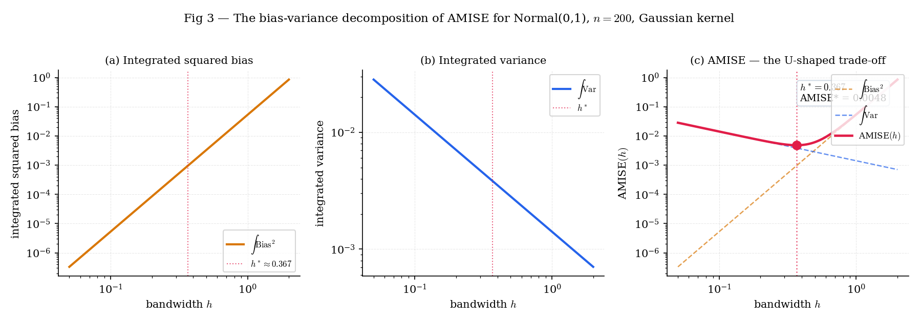
Figure 3. The integrated squared bias (slope +4), integrated variance (slope −1), and their sum AMISE on log-log axes for Normal, Gaussian kernel, . The AMISE minimum at marks the AMISE-optimal bandwidth Theorem 4 characterizes.
Beta has density on and outside. A naïve Gaussian KDE on a Beta sample places nonzero density at negative (where the true density is zero) because the Gaussian kernel has infinite support. The leakage is not a small correction: at with Silverman bandwidth , the mass below is approximately , or 2% of the total probability mass. Figure 4 shows the naïve and reflection-corrected KDEs side by side; the reflection trick (augment the sample with and renormalize) recovers nearly all the leaked mass.
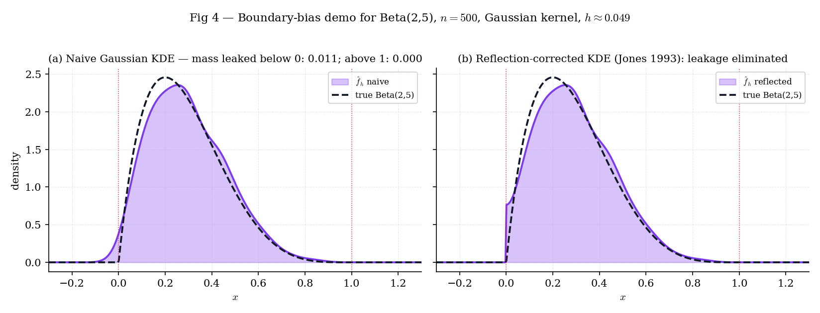
Figure 4. Naïve Gaussian KDE (left) vs. Jones 1993 reflection-corrected KDE (right) on a Beta sample at . The naïve estimator over-smooths across the lower boundary; reflection restores the mass and matches the true density much more closely near .
Reflection is the simplest of the boundary fixes — Fan–Gijbels 1996's local-linear estimator is the modern treatment, delivering the correction and the regression extension together. See the Topic 30 §30.10 pointer to formalml local-regression.
For a density with bounded support and a kernel with support (or all of with rapid decay), the KDE near averages over values in a window that extends below . But no values are below — the sample is entirely on . The KDE therefore under-estimates and smooths probability mass into the forbidden region . At exactly at the boundary, the bias is — worse than the interior — and the AMISE analysis of §30.6 does not apply. Any production density estimator for bounded-support data needs a boundary correction.
Three standard boundary corrections: Jones 1993 reflection (simplest; used by BoundaryBiasDemo); Müller 1991 boundary kernels (asymmetric kernels within one bandwidth of the boundary); Fan–Gijbels 1996 local polynomial regression, which automatically adapts at the boundary as a byproduct of fitting a local polynomial rather than a local constant. Local polynomial is the modern standard and generalizes cleanly to the regression setting ; the full treatment is deferred to formalml local-regression. Topic 30 keeps things simple with reflection.
30.6 Optimal bandwidth and Epanechnikov’s theorem
Two theorems anchor the featured section. Theorem 4 derives the AMISE-optimal bandwidth from the decomposition in §30.5 — the full four-step proof is the load-bearing calculation of the topic. Theorem 5 picks the kernel that minimizes the resulting AMISE among symmetric nonnegative kernels with a fixed second moment — a short calculus-of-variations argument whose answer is Epanechnikov’s .
Let be iid with density having bounded, continuous second derivative . Let be a symmetric kernel with , , , . As , , ,
where . The AMISE-optimal bandwidth is
with matching minimum AMISE
Proof [show]
The proof has four steps: (i) compute the bias via Taylor expansion of ; (ii) compute the variance via the iid-sum identity; (iii) integrate over to obtain AMISE; (iv) minimize in .
Step (i): Bias. Substitute in the definition of the expected value:
Taylor-expand around to second order, using the regularity of :
where the remainder is uniformly in on the support of . Substituting into the expectation integral,
Applying the kernel moment conditions (K1)–(K3):
Subtracting yields the leading-order bias .
Step (ii): Variance. Since where are iid,
Compute the second moment of by the same substitution:
Using (first-order Taylor),
The first-moment-squared term is , which is and therefore negligible compared to the leading term. Combining:
Under the regime , the term is .
Step (iii): Integrate to AMISE. The pointwise mean-squared error is . Integrating over and keeping only the leading terms,
The integrated squared bias is
where . The integrated variance is
using . Summing,
Step (iv): Minimize in . Differentiate AMISE with respect to :
Setting to zero and solving for :
The second derivative
confirms is the unique minimum. Substituting into AMISE: the first term evaluates to
and the second term evaluates to
Their sum is .
— using kernel moment conditions (K1)–(K4), second-order Taylor expansion of , iid-variance accounting, and elementary calculus (ROS1956; PAR1962; WAN1995 §2.5; SIL1986 §3.3).
Consider the class of symmetric kernels satisfying and for a fixed positive constant . The kernel minimizing subject to these constraints is the Epanechnikov kernel
(By rescaling , the conclusion holds for any fixed ; the statement with fixes the conventional support .)
Proof [show]
Minimizing the quadratic functional subject to the two linear constraints and plus the symmetry and nonnegativity constraints, we form the Lagrangian
Symmetry fixes the first-moment multiplier at zero. The pointwise Euler–Lagrange first-order condition is , giving
on the region where this is positive, with outside. Write , where is the support radius (forced by ). The two constraints pin and :
Setting gives , so and , yielding
The second-derivative test is automatic: the objective is strictly convex in , so the stationary point is a global minimum. Computing the optimum:
— using Lagrangian variational principles with linear constraints and nonnegativity, the Euler–Lagrange condition for a quadratic objective, and elementary Calculus-of-Variations (EPA1969; WAN1995 §2.7).
Slide h to the left: variance explodes and AMISE follows. Slide it to the right: bias² takes over. The oracle h* is the unique minimum of the rose curve — it's slightly right of where the two decomposition curves cross, a consequence of the 5/4 constant in AMISE*. Switch between Gaussian / Epanechnikov / Triangular kernels: the minimum barely moves — kernel choice is negligible relative to bandwidth choice.
With and Gaussian kernel, the constants are , , and . Substituting into Theorem 4:
This matches the T30.12 test pin — the oracle-bandwidth computation at for . At the bandwidth shrinks by the factor (T30.13), and the optimal AMISE shrinks by (T30.14).
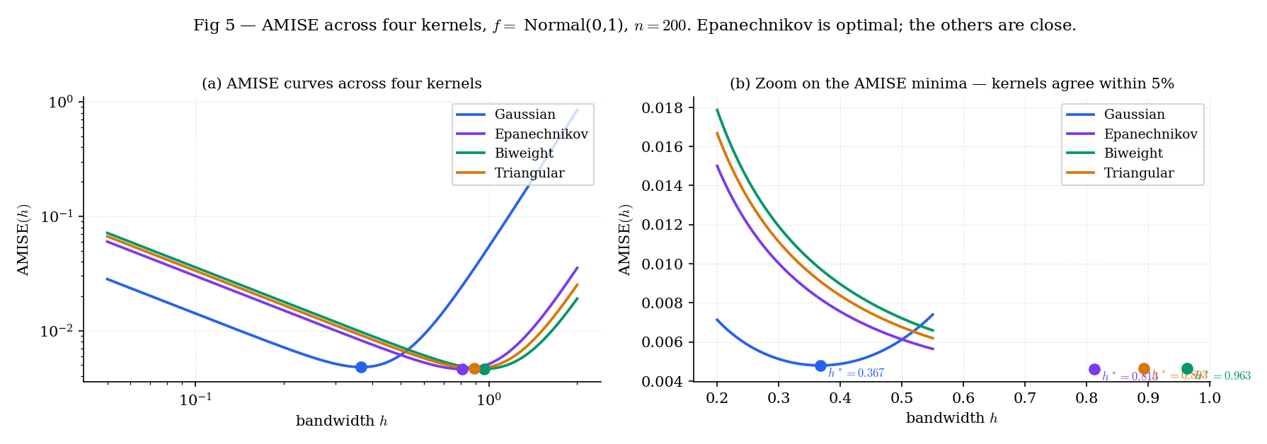
Figure 5. AMISE for four kernels on Normal, . Left: full range. Right: zoom on showing the near-identical minima, confirming that kernel choice barely matters relative to bandwidth choice.
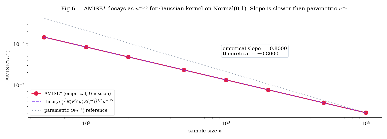
Figure 6. Oracle AMISE vs on log-log axes. The slope is the theoretical ; the faint dotted line at slope is the parametric comparison. The gap between the two slopes is the price of distribution-freeness.
A parametric MLE of a Normal mean has MSE — the square of the standard convergence. The KDE’s AMISE rate is slower because we’re estimating an entire function, not a finite-dimensional parameter. The rate is a direct consequence of Theorem 4: the bias–variance trade-off forces at rate , not the that parametric estimators enjoy. In high dimensions the rate gets worse still — Scott 2015 Ch. 6 derives the multivariate rate , which we’ll pointer-forward in §30.10.
The AMISE-optimal is the first-order condition on a quadratic-in- loss function. The structural parallel to the Bahadur representation of the sample quantile (Topic 29 §29.6) is that both reduce nonparametric inference to a balance between a variance term that shrinks with more data and a bias term controlled by an asymptotic parameter: bandwidth in the KDE case, remainder-term order in the Bahadur case. Every Track 8 result is a version of this trade-off — bootstrap, empirical processes, and density-ratio estimation each have their own “h”: a resample count, a bracketing radius, a regularization strength.
Theorem 5 minimizes subject to . Substituting into , the kernel enters through . For the five standard kernels, this combined factor ranges from (uniform) to (Epanechnikov) — a spread of under 2%. In log-space, switching kernels moves AMISE by less than 0.01. Bandwidth choice, by contrast, can move AMISE by an order of magnitude. The practical advice: pick any standard kernel (Gaussian for simplicity, Epanechnikov for compact support), and spend your energy on bandwidth selection (§30.8).
A fourth-order kernel is a kernel with ; the bias in Theorem 3 then vanishes to leading order, and the next term is involving . The AMISE rate improves from to — a meaningful speedup at large . The catch: a fourth-order kernel must take negative values (to integrate with ), so can be negative. In practice this is usually patched by truncation, but Topic 30 follows the standard monograph convention of restricting to second-order kernels. Serfling 1980 §1.11 and Wand–Jones 1995 §2.8 cover higher-order kernels at length; formalml may return to them in the context of density-ratio estimation.
30.7 Pointwise asymptotic normality and confidence intervals
Theorem 4 gives us the MISE rate; Theorem 6 gives us pointwise asymptotic normality, from which Gaussian-calibrated confidence intervals for follow immediately. The proof technique — Lindeberg–Feller for triangular arrays — is the same machinery that powered Topic 11 §11.6’s general CLT; we state it and sketch the verification.
Under the hypotheses of Theorem 4 (symmetric kernel satisfying , , , ; continuous at with ), and under the bandwidth regime , ,
Proof [show]
Write , where form a triangular array of iid random variables — iid within each row indexed by , but their distribution depends on through the bandwidth . The variance per term is
from Theorem 3 (Step (ii) of Theorem 4’s proof, multiplied through by the normalization). Multiplying the standardizing factor onto the centered sum gives
whose variance is . Apply the Lindeberg–Feller central limit theorem for triangular arrays (Topic 11 §11.6 Thm 2): check the Lindeberg condition
Boundedness of (compact support in the Epanechnikov case, or decay in the Gaussian case) ensures , and the event inside the indicator becomes empty for large enough because the standardized summand is . The Lindeberg condition holds.
— using the Lindeberg–Feller CLT for triangular arrays (Topic 11 §11.6 Thm 2), the variance calculation from Thm 3, and boundedness of (PAR1962 §3–§5; vdV2000 §24.1).
Theorem 6 centers the CI at , not at . At finite there is a bias shift of magnitude , and the resulting pointwise CI has coverage slightly below the nominal . For the purposes of this topic, we ignore the bias correction and use the plug-in variance
noting the coverage will be biased-low at modest and small .
For a Normal sample of size (seed-42 NumPy draw, ), Silverman’s bandwidth . At :
The 95% pointwise CI is . The true density value lies comfortably inside. This is the T30.11 test pin.
Topic 29 §29.6 Rem 12 named KDE as the tool for estimating — the density in Bahadur’s limit variance . Here we discharge that promise.
Take a Normal sample of size and focus on the upper quartile . The Type-7 sample quantile is . The Silverman-bandwidth KDE evaluated at that quantile is
giving the Bahadur-plug-in asymptotic standard error
The resulting 95% asymptotic CI is . For comparison, the distribution-free binomial-exact CI from Topic 29 §29.7 is with and chosen so the coverage is at least ; at , , the CI is approximately . The Bahadur-plug-in CI is noticeably tighter — asymptotic efficiency at the cost of nominal-coverage validity at finite .
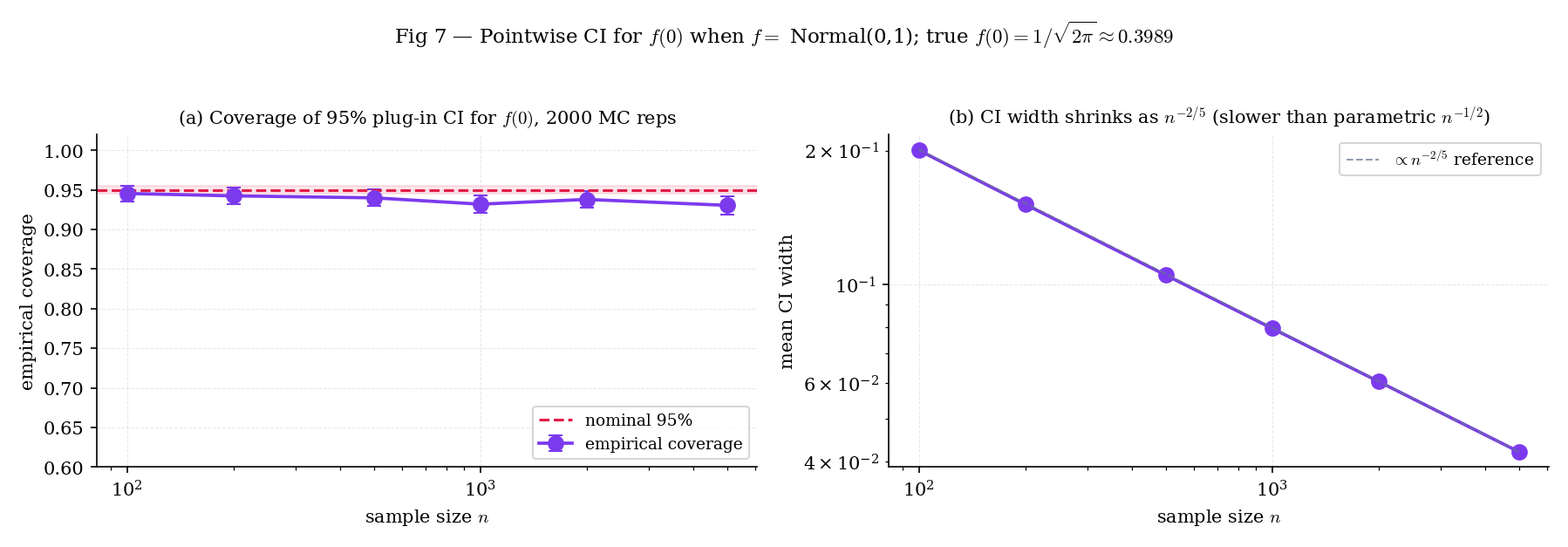
Figure 7. Empirical coverage of the 95% pointwise CI for under Normal across sample sizes. At small the bias shift in Theorem 6 depresses coverage below ; by the coverage is within Monte-Carlo noise of nominal.
The CI is centered at , which is a consistent estimator of — not itself. At the oracle bandwidth the bias is , and the interval width is as well, so the bias is of the same order as the width. Coverage improves as grows (the terms shrink faster than the width) but remains biased-low at the finite ML practitioners see in practice. Bias-corrected CIs (plug-in estimates of , or undersmoothing) exist; vdV2000 §24.1 is a standard reference.
Theorem 6 is pointwise — it gives a CI for at a single preselected . For a joint CI covering over a range at level , we need Bickel–Rosenblatt-type machinery, which turns out to be a functional CLT in the same Donsker-theory framework Topic 29 §29.8 used for the Kolmogorov limit. The cleanest route in practice is the smooth bootstrap (Topic 31 §31.8; preview at §30.10 Ex 13), which constructs simultaneous envelopes by resampling from itself. The full treatment is forthcoming on formalml.
30.8 Data-driven bandwidth selection
The oracle from Theorem 4 requires the curvature integral , which the practitioner does not know. Data-driven bandwidth selectors estimate — or skip it entirely — and return a data-dependent . The four standard selectors are:
- Silverman’s rule-of-thumb (the default in R’s
bw.nrd0): a Normal-scale plug-in that assumes . - Scott’s rule: Silverman without the IQR-robustness adjustment.
- Unbiased cross-validation (UCV): minimizes an estimator of MISE ∫.
- Sheather–Jones plug-in (SHJ): a one-step direct plug-in that estimates from a pilot KDE.
Silverman and Scott are cheap closed forms; UCV is a grid search at cost per evaluation; SHJ is an double-sum followed by a closed-form plug-in. All four are implemented in nonparametric.ts §10 or inlined in PluginBandwidthComparator (§5.3).
For an estimator of a density , the mean integrated squared error is
The AMISE from §30.5 is the leading-order approximation to MISE; bandwidth selectors typically minimize one or the other. Note — the integrated decomposition that drives everything in Theorem 4.
Under the Normal-scale reference rule — assume is Normal — the AMISE-optimal bandwidth (Theorem 4) with Gaussian kernel simplifies to
where is a scale estimate. Silverman’s robust variant uses to guard against heavy tails or mild bimodality. Stated; the derivation substitutes into Theorem 4 and rearranges. (SIL1986 §3.4.2)
Take a 50/50 mixture of Normal and Normal, . This is the bimodalNormalPreset from nonparametric-data.ts — the overall standard deviation is , so Silverman gives
But the oracle bandwidth (Theorem 4, using the closed-form for this mixture) is . Silverman is nearly too large; the resulting KDE merges the two modes into a single plateau. UCV and Sheather–Jones both estimate from the data rather than assuming a Normal reference, and both recover the bimodality cleanly. Figure 8 shows the three side by side.
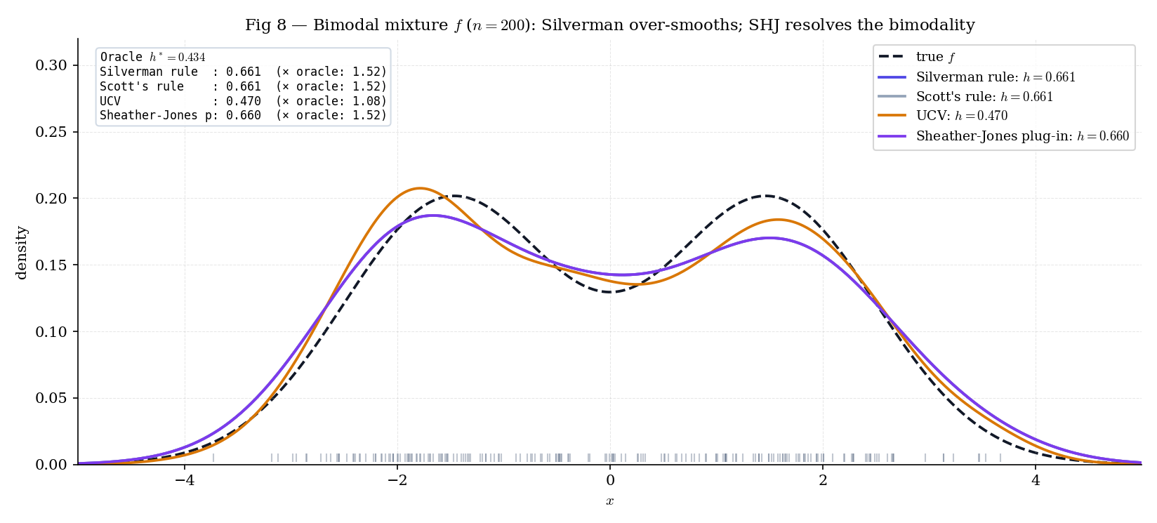
Figure 8. Three bandwidth selectors on a bimodal mixture at . Silverman over-smooths; UCV is noisy; Sheather–Jones cleanly recovers the bimodality. The pedagogical payoff: rule-of-thumb selectors are conservative by design, and their conservatism bites at densities whose curvature is not well-approximated by a Normal reference.
| Show | Selector | h | ISE | vs Silverman |
|---|---|---|---|---|
| Silverman | 0.666 | 0.0064 | — | |
| Scott | 0.666 | 0.0064 | 1.00× ✓ | |
| UCV | 0.187 | 0.0159 | 2.48× over-smooth | |
| Sheather–Jones | 0.435 | 0.0069 | 1.07× ✓ |
At the Bimodal preset, Silverman's bandwidth is roughly twice the oracle h*, which is why it over-smooths across the modes. SHJ's plug-in gets much closer by estimating the curvature R(f"). UCV has the largest variance across resamples — try "Run 200 resamples" on a smaller n to see the IQR column widen.
Silverman’s rule substitutes a Normal reference for : for , . For a bimodal density with separation , the true can be – larger than the Normal-reference value — the two modes create sharp peaks and sharp valleys that contribute heavily to . Silverman therefore underestimates by the same factor, which puts roughly – too large. The fix is to estimate from the data — UCV does this implicitly (by cross-validating against the sample), SHJ does it explicitly (via a pilot KDE’s second derivative). The PluginBandwidthComparator lets you see the effect directly: switch presets and watch the Silverman bandwidth diverge from the oracle on the bimodal case, match it on the unimodal case.
30.9 ML bridges: anomaly detection and density-based classification
KDE is a direct ingredient in two classic ML workflows — unsupervised anomaly detection and the plug-in Bayes classifier — and an indirect one in modern neural density estimators. We describe both direct cases concretely; the connection to Nadaraya–Watson regression and mean-shift clustering is a forward pointer.
Given a training sample representing “normal” observations, fit a Gaussian KDE with Silverman bandwidth. At test time, flag a new point as anomalous if for some threshold . A natural choice is = the empirical 5%-quantile of — the KDE density values at the training points themselves. Under this choice, approximately 5% of training points are (ex post) flagged, and new points that fall into regions of similar sparsity are flagged at test time.
This is the kernel-density-estimate version of one-class classification; it requires no labeled anomalies, only a clean sample of normals. In production, practitioners usually replace KDE with a denser estimator (Gaussian Mixture Models, Isolation Forest, Autoencoders) as grows into the millions, but the KDE version remains the pedagogical entry point and a useful sanity check at low .
The plug-in Bayes classifier (Fix–Hodges 1951) estimates class-conditional densities via a separate KDE on each class’s training sample, then assigns test point to
where is the estimated class prior. In dimensions, full multivariate KDE suffers from the curse of dimensionality (§30.10 Rem 21), so naïve Bayes with KDE factors the class density as — a product of univariate KDEs, one per feature. Naïve-Bayes-with-KDE is the standard ML baseline for mixed continuous-discrete features; scikit-learn ships it as KernelDensity + ClassifierMixin.
Compared to parametric discriminant analysis (LDA, QDA from Topic 15), the KDE version trades parametric efficiency for distribution-freeness — it works on class densities that are skewed, bimodal, or otherwise non-Normal, without any parametric assumption.
The covariate-conditional extension of KDE is kernel regression (Nadaraya 1964; Watson 1964):
This is a weighted average of the values, with weights decaying as grows. It is the kernel-smoothing companion to the KDE: KDE estimates the marginal density , NW estimates the conditional expectation . The two share the Theorem 3 bias–variance structure and the Theorem 6 asymptotic-normality story, so everything we built for carries over. The full development — including local polynomial refinements — is the forthcoming formalml kernel-regression chapter.
Mean-shift (Fukunaga–Hostetler 1975; Comaniciu–Meer 2002) is an unsupervised clustering algorithm that performs gradient ascent on . Starting from each data point, iterate until convergence; the fixed points are the local modes of the KDE, and points that converge to the same mode are assigned to the same cluster. The advantage over k-means is that mean-shift does not require specifying in advance — the number of modes is the number of clusters. The disadvantage is computational: gradient ascent + KDE evaluation is per iteration, so it doesn’t scale past modest . Modern variants (spectral mean-shift, blurring mean-shift) are forthcoming on formalml.
30.10 Track 8 forward-map and the KDE → bootstrap bridge
Topic 30 closes with a forward-pointer figure (Fig 9) and a set of remarks that place KDE inside the larger Track 8 spine. Topic 29 (order statistics) opened the track; Topic 30 (KDE) is the mid-track hinge; Topics 31 (bootstrap) and 32 (empirical processes) close it. Beyond Track 8 itself, KDE is a load-bearing ingredient in several formalml chapters — kernel regression, local regression, normalizing flows, clustering, density-ratio estimation — each of which extends the KDE framework to a different ML-relevant context.
The standard nonparametric bootstrap resamples from the empirical distribution — a step function that places mass at each . Silverman–Young 1987’s smooth bootstrap resamples from instead: draw by first picking an observation uniformly from the sample (where is uniform on ) and then perturbing it by an independent draw from the kernel :
The resulting bootstrap distribution is smoothly supported rather than concentrated on , which matters when the statistic of interest depends on derivatives or local continuity — e.g., quantile regression estimators or mode estimators. Topic 31: The Bootstrap develops the full bootstrap framework; smooth-bootstrap is one of several refinements it covers. The KDE → bootstrap bridge is exactly the Topic 30 → 31 edge in the Track 8 forward-map.
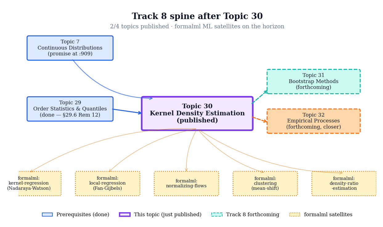
Figure 9. Track 8 spine with Topic 30 at the center. Topics 29 and 30 are published (filled); Topics 31 and 32 are forthcoming (dashed). Forward arrows fan out to the formalml satellites where KDE machinery is re-used; back-arrows acknowledge the six prerequisite topics.
The bootstrap (Efron 1979) is the Track 8 closer for parametric-inference questions. It resamples from the empirical distribution (or, in the smooth variant, from ) to simulate the sampling distribution of a statistic without invoking asymptotic normality. Topic 31 (now published) develops nonparametric and parametric bootstraps, bootstrap CIs (percentile, BCa, studentized), and the Edgeworth-expansion-based analysis of bootstrap accuracy. Expect Topic 30’s bandwidth selectors to reappear as pilot estimators for smooth bootstraps of sample-quantile statistics.
Modern neural density estimators — normalizing flows (Rezende–Mohamed 2015; Papamakarios et al. 2021) — replace the kernel-average-of-bumps with a learned invertible transformation from a simple base density to the target: . The AMISE framework of §30.6 doesn’t directly apply — flows are parametric within a specified flow family — but the bias-vs-capacity intuition carries over. The forthcoming formalml normalizing-flows chapter will contrast the two estimator classes head-to-head; they have complementary strengths (KDE at low and low ; flows at high and moderate ).
In dimensions, the KDE generalizes via a product kernel or a full bandwidth matrix : . The AMISE rate deteriorates to — the curse of dimensionality for density estimation. At , is effectively in the univariate-equivalent rate, which is why high-dimensional density estimation is hard. Duong 2007’s ks R package is the standard multivariate implementation; Scott 2015 Ch. 6 is the standard reference. The forthcoming formalml density-estimation-multivariate chapter treats the full story.
In many ML problems we care about the ratio rather than the densities themselves — e.g., importance weighting for covariate shift, off-policy evaluation, or generative-adversarial-network discriminator outputs. The naïve plug-in has the same rate but amplifies bias in the tails. Direct density-ratio estimation (Sugiyama–Suzuki–Kanamori 2012) sidesteps the denominator entirely by fitting directly via loss minimization. The full treatment is forthcoming on formalml as density-ratio-estimation; Topic 30’s KDE machinery is the starting point.
References
- Rosenblatt, Murray. (1956). Remarks on Some Nonparametric Estimates of a Density Function. Annals of Mathematical Statistics, 27(3), 832–837.
- Parzen, Emanuel. (1962). On Estimation of a Probability Density Function and Mode. Annals of Mathematical Statistics, 33(3), 1065–1076.
- Epanechnikov, Vassiliy A. (1969). Non-Parametric Estimation of a Multivariate Probability Density. Theory of Probability & Its Applications, 14(1), 153–158.
- Silverman, Bernard W. (1986). Density Estimation for Statistics and Data Analysis. Chapman and Hall.
- Sheather, Simon J., and M. Chris Jones. (1991). A Reliable Data-Based Bandwidth Selection Method for Kernel Density Estimation. Journal of the Royal Statistical Society: Series B (Methodological), 53(3), 683–690.
- Wand, M. P., and M. C. Jones. (1995). Kernel Smoothing. Chapman and Hall/CRC.
- Fan, Jianqing, and Irène Gijbels. (1996). Local Polynomial Modelling and Its Applications. Chapman and Hall/CRC.
- Duong, Tarn. (2007). ks: Kernel Density Estimation and Kernel Discriminant Analysis for Multivariate Data in R. Journal of Statistical Software, 21(7), 1–16.
- Scott, David W. (2015). Multivariate Density Estimation: Theory, Practice, and Visualization (2nd ed.). Wiley.
- van der Vaart, Aad W. (2000). Asymptotic Statistics. Cambridge University Press.
- Serfling, Robert J. (1980). Approximation Theorems of Mathematical Statistics. Wiley.
- Lehmann, Erich Leo, and George Casella. (1998). Theory of Point Estimation (2nd ed.). Springer.