Multiple Testing & False Discovery
When one test becomes many: controlling FWER via Bonferroni, Holm, and the closed-testing principle; controlling FDR via Benjamini–Hochberg; adaptive q-values via Storey; and the dual Bonferroni / Šidák simultaneous confidence intervals that close Track 5.
20.1 The FWER Explosion Problem
A single hypothesis test at level makes the following contract with a scientist: if the null is true, the probability of a false rejection is at most . Twenty replications of the same experiment, each analyzed with the same level- test, would make twenty independent such contracts — and on average, one of them would falsely reject the null. That is already uncomfortable. In modern practice, is not twenty; it is twenty thousand (GWAS), or two hundred thousand (high-throughput imaging), or — most commonly — the number of coefficients in a regression multiplied by the number of pre-registered contrasts multiplied by the number of subgroup analyses. The per-test guarantee degrades catastrophically with , and without an adjustment, "" stops meaning what the untrained reader assumes.
The simplest quantification of the degradation assumes independence between the tests. If each test has Type I error exactly under the null, and all nulls are true, then
This quantity is the family-wise error rate (FWER) under the global null. For small the Taylor expansion gives , which is the same answer the union bound returns unconditionally (no independence required). Both bounds explode with : at the table below is unforgiving.
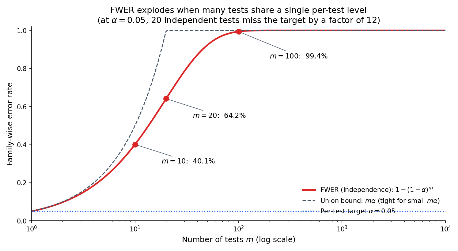
A product team runs twenty simultaneous A/B tests on unrelated features, each at level . None of the twenty has a true effect — the global null holds. The probability that at least one test falsely flags its feature as significant is . A team that deploys whichever features cross the threshold will, in expectation, ship at least one null feature in this batch. Doing this every quarter across a company compounds the effect: after four quarters, the probability of never having shipped a null feature is .
A GWAS tests common variants against a trait. The union-bound control at gives a per-test threshold of — the number that has become the de facto field standard for “genome-wide significance.” It is exactly the Bonferroni correction of §20.4 applied to the GWAS scale. The FDR-controlled threshold for the same data is typically two or three orders of magnitude less stringent (§20.7 Ex 8), which is why BH-based analyses routinely identify hits that genome-wide-significance analyses miss.
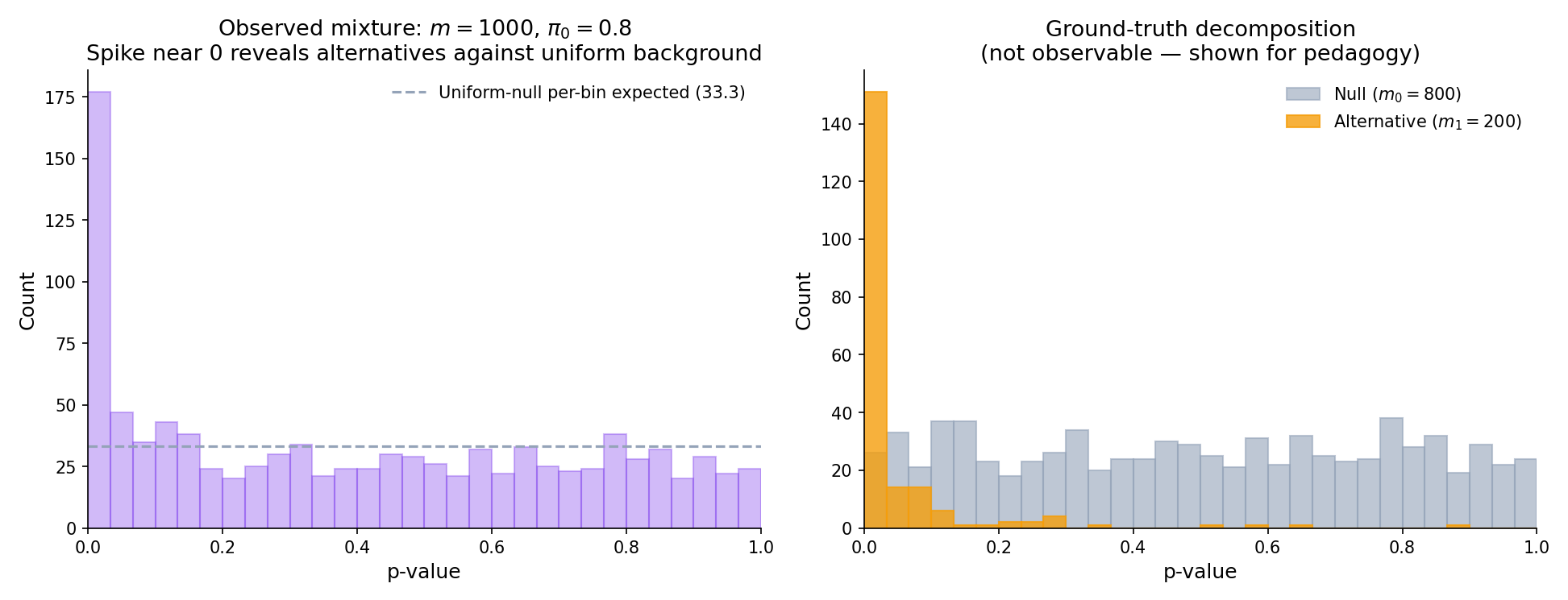
A multiple-testing problem consists of hypotheses with null distributions and test statistics producing p-values . Let denote the subset of indices where is true (the true nulls), with and the count of true alternatives. Write for the true null fraction.
A multiple-testing procedure is a function returning the set of rejected hypotheses. Counts of interest: (total rejections), (false rejections), (true rejections); by construction . Throughout the topic, denotes the rejection set and its cardinality.
Bonferroni’s correction — apply each test at level — is the canonical fix and will be formalized in §20.4. It works, but it is uniformly conservative: the FWER it actually achieves under the global null is at most , often much less. The rest of this topic is about more powerful procedures that retain the FWER guarantee (Holm, Hochberg, closed testing) or relax it to the weaker-but-often-preferred FDR guarantee (BH, BY, Storey). The pedagogical arc: is the floor, not the ceiling.
The exact formula uses independence; the union bound does not. Under positive dependence — the typical regime for correlated tests in an A/B platform or for linkage-disequilibrium-correlated SNPs in a GWAS — the exact FWER is smaller than the independent-case formula (the false rejections tend to cluster). Under negative dependence, it can be larger, but negative dependence is rare in practice. The upshot: is a safe universal upper bound; is tight under independence; the truth-under-positive-dependence is somewhere in between.
20.2 The Closed-Testing Principle
Before stating Bonferroni, we describe the organizing scaffold that derives Holm (and many other step-down procedures) from a single principle. Closed testing (Marcus, Peritz, and Gabriel 1976) is a two-step recipe: test every non-empty intersection hypothesis at level ; reject in the final procedure iff every intersection containing rejects. This simultaneously achieves strong FWER control — regardless of the individual tests’ dependence structure — and, when the base tests are chosen appropriately, produces procedures strictly more powerful than single-step corrections.
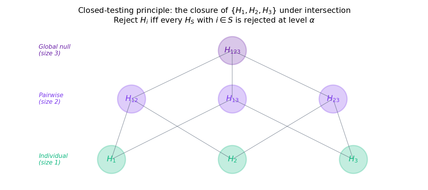
Let be a level- test of for every non-empty . Define the closed procedure to reject iff rejects for every . Then for any true-null configuration :
No dependence assumption on the individual test statistics is required.
The proof is a one-line observation: a false rejection of any with requires to reject, and is a level- test of the true null , so this has probability . Full exposition and the induction argument that specializes this to Holm are in : §9.1. We will not reproduce it; for Topic 20 the role of closed testing is organizational — it is the lens through which Holm (§20.5) and Hochberg (§20.5) become instances of a single construction rather than ad-hoc step-down rules.
The theorem above says “pick level- tests of every intersection and combine them correctly.” It does not tell you which tests to pick. Bonferroni-based intersection tests (reject iff ) give the Holm procedure. Fisher-combination intersection tests (reject iff exceeds a critical value) give a different, often more powerful closed procedure. Simes-combination tests give Hochberg. The space of reasonable closed procedures is large; practitioners gravitate to Holm because it is parameter-free and always-valid.
The full proof machinery — proving strong control and showing Holm is the closed procedure with Bonferroni intersection tests — takes roughly 15 additional lines of careful indexing. It adds no conceptual insight beyond what the one-line sketch above already conveys, and it distracts from the BH proof in §20.7, which does deserve a full derivation. Closed testing is the scaffold; the specific procedures we prove correct (Bonferroni, Holm, BH) are the load-bearing walls.
20.3 Family-Wise Error Rate: The FWER Paradigm
For a multiple-testing procedure producing rejection set on data with true-null configuration , the family-wise error rate at is
A procedure controls FWER at level if for every configuration .
A procedure controls FWER in the weak sense if only when (the global null — every true). It controls FWER in the strong sense if for every , including the partial-null configurations where some are true and some are false.
Strong control is what practitioners want: the guarantee should hold whether or not the alternatives are real. Weak control is an academic fallback. Every procedure in this topic controls FWER or FDR in the strong sense unless explicitly noted.
At FWER collapses to the per-test Type I error of : . FWER is the multi-hypothesis generalization: it replaces “probability this particular test falsely rejects” with “probability any of the tests falsely rejects.” The two notions agree at and diverge sharply for large , as §20.1 Fig 1 shows.
Holding each test’s nominal level fixed, controlling FWER at level forces each individual test to use a smaller effective . Smaller per-test level means smaller per-test power. The trade-off is quantitative: under Bonferroni at global , a test of a single alternative with effect size that had power at with retains only power at and at — a dramatic loss. The FDR framework of §20.6 sacrifices some of FWER’s protection to claw back this power, and is the right tool whenever false discoveries (rather than any false rejection whatsoever) are the cost metric.
20.4 Bonferroni and Šidák
Bonferroni is the starting point: reject iff . It controls FWER without any dependence assumption and its proof is immediate.
The Bonferroni procedure rejects iff . It controls FWER at level in the strong sense under any joint dependence structure among the test statistics.
Proof Proof 1 — Bonferroni FWER control [show]
Let be the number of false rejections. The event equals the union . Applying the union bound (see : ):
The first inequality is the union bound; the second uses that each for is stochastically at least Uniform(0, 1), so . No independence is needed. ∎ — using Boole’s inequality.
Proof 1 is three lines because Bonferroni is morally the union bound. The trade-off is that it uses the union bound even when better control is possible — independence-based procedures (Šidák) or step-down procedures (Holm) achieve larger per-test thresholds while retaining FWER control.
Suppose the test statistics are independent under . Then the Šidák procedure — reject iff — controls FWER in the strong sense at exactly when and at most otherwise.
Under independence, Šidák’s threshold is slightly larger than Bonferroni’s ( for every , with equality in the limit ), but the gap is tiny: at and the thresholds are (Šidák) vs (Bonferroni), a difference. Šidák is strictly more powerful when independence holds, but practitioners typically prefer Bonferroni because its universal validity (no dependence assumption) outweighs the marginal power gain when independence is questionable. Stated without proof; see : .
Per-test threshold . A test with a -value of — significant at the level for a single test — is not significant under Bonferroni. The union-bound-guaranteed FWER is at most ; under independence the exact FWER is , slightly below the bound.
For essentially every routine application, the two give numerically indistinguishable thresholds. The deciding factor is the dependence story: Bonferroni is correct under any dependence, Šidák is exact under independence and conservative-then-liberal under positive-then-negative dependence. Textbook tables default to Bonferroni; the software outputs often default to Šidák (e.g., R’s p.adjust(method = 'bonferroni') vs the closely-related Šidák implementations). The practical answer is almost always the same hypothesis-level decisions.
The Bonferroni intersection test — “reject iff ” — is itself a valid level- test of the intersection hypothesis . Applying closed testing with Bonferroni intersection tests produces exactly the Holm step-down procedure of §20.5 (LEH2005 §9.1). This is the cleanest way to see why Holm strictly dominates Bonferroni: the closed procedure exploits the fact that once a hypothesis is rejected, the remaining intersections shrink, and subsequent Bonferroni thresholds become less stringent.
20.5 Holm’s Step-Down and Hochberg’s Step-Up
Holm’s step-down procedure is uniformly more powerful than Bonferroni: every rejection Bonferroni makes, Holm also makes; and Holm additionally rejects hypotheses with -values up to (the least-stringent threshold, at the end of the step-down walk). It preserves Bonferroni’s strong FWER control without requiring independence.
Order the -values ascending: . Let be the smallest rank such that (set if no such exists). The Holm procedure rejects the hypotheses corresponding to . This controls FWER at level in the strong sense under any joint dependence structure.
Proof Proof 3 — Holm FWER control (induction on rank order) [show]
Let be the true-null configuration with and let be the smallest rank (in the overall ordering of ) at which some true null appears. Equivalently, : the first positions in the ordering must be alternatives (if every null is larger than every alternative, which is the worst case for Type I; otherwise is smaller, which only makes a false rejection require a smaller ).
We show that — the probability that Holm falsely rejects at least one true null — is at most . A false rejection requires Holm to walk past step , which requires . At rank , exactly of the remaining -values are true nulls. The smallest of those null -values — call it , the first-order statistic of the null -values — is at most . So
The first-order statistic of null -values, each stochastically at least Uniform(0, 1), is at most with probability at most by the union bound:
Combining the two displays: . No dependence assumption is required because every inequality used is the union bound applied to events on a fixed set of null-indexed -values. ∎ — using induction-on-rank + union bound; HOL1979.
The proof shows why Holm dominates Bonferroni: Bonferroni uses the union bound once at threshold ; Holm uses it at threshold , which is larger when (i.e., whenever there are real alternatives). The step-down structure is the device that lets the threshold depend on the number of surviving hypotheses.
Order the -values ascending. Let be the largest rank such that (set if no such exists). The Hochberg procedure rejects . This controls FWER at level under independence or positive regression dependence (PRDS).
Hochberg uses the same threshold function as Holm — at rank — but walks the ranks in the opposite direction (from largest -value down to smallest, stopping at the first that passes) rather than step-down (stopping at the first that fails). It is uniformly more powerful than Holm when independence holds, at the cost of requiring that assumption. Stated without proof; see : .
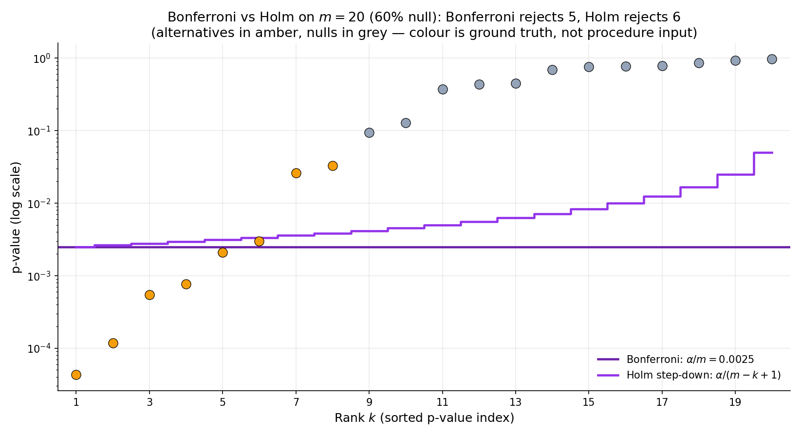
Suppose 3 of the 20 -values are below : specifically , and . Bonferroni rejects the first three. Holm: (pass), (pass), (pass), ? No — , so Holm stops and rejects . Same rejections as Bonferroni in this case, but Holm’s threshold at rank 4 is less stringent than Bonferroni’s constant , so if had been, say, , Holm would additionally reject it while Bonferroni would not.
Take , , ordered -values . Holm: (pass), (pass), ? No — , stop. Rejects 2. Hochberg: start at ? Yes — reject all 5. The same inputs give very different answers: Hochberg’s step-up detects the global pattern (“all five look moderately small”) while Holm’s step-down commits early. Hochberg is valid under independence; Holm makes no such assumption.
Open the explorer below; set , ; sweep from (dense signal) to (sparse). At Holm and BH both recover most of the 100 alternatives; Bonferroni recovers perhaps . At Holm and Bonferroni converge (both at rejections) while BH retains nearly all of the 2 expected true alternatives. This is the core FDR-vs-FWER story and it is best seen interactively.
| Procedure | R | V | S | FDP | Power |
|---|---|---|---|---|---|
| Bonferroni | 6 | 0 | 6 | 0.0% | 30.0% |
| Holm | 6 | 0 | 6 | 0.0% | 30.0% |
| Benjamini–Hochberg | 15 | 0 | 15 | 0.0% | 75.0% |
R = total rejections, V = false rejections (from nulls), S = true rejections (from alternatives). FDP = V/R; power = S/m₁.
Default exploration configuration; realistic for behavioral-science multi-test scenarios.
Example p-value (first shown): 0.0212. Click Resample to draw a fresh p-value vector at the same (m, π₀, δ, α); the relative ranking of procedures stays stable, but individual rejects shift.
The step-down structure guarantees that Holm’s rejection set contains Bonferroni’s: if , then a fortiori . So every Bonferroni rejection is a Holm rejection, and Holm potentially adds more as the rank grows. There is no regime where using Bonferroni instead of Holm is better; use Holm by default.
Hochberg’s step-up is strictly more powerful than Holm’s step-down under independence, but not under arbitrary dependence. In GWAS (LD-correlated tests) and most A/B test multiplicity, positive dependence holds and Hochberg is safe and preferred. In high-dimensional regression where the design matrix is ill-conditioned, dependence structure can be complex and Holm is the conservative default.
Applying the closed-testing scaffold (§20.2 Thm 0) with Bonferroni intersection tests — “reject iff ” — produces exactly the Holm step-down procedure. This is : §9.1 Thm 9.1.2. The derivation explains why Holm’s rank-dependent threshold is : at step , the remaining candidate intersection has size , and its Bonferroni threshold is .
No. Holm is admissible among step-down procedures that control FWER under arbitrary dependence (you can’t uniformly improve it), but it is not UMP. The closed-testing framework allows other intersection-test choices (Fisher combination, Simes, …) that can dominate Holm on specific alternative configurations while still controlling FWER in the strong sense. Procedure choice depends on the expected dependence and signal structure. See LEH2005 §9.1 for the admissibility theorems.
20.6 False Discovery Rate: A New Error Metric
Benjamini and Hochberg (1995) observed that FWER control is often overkill. In a genome-wide association study with tested SNPs, a practitioner flags as significant. They are content if of those are false positives (10% FDP) — that is the rate at which follow-up experiments will fail. They do not specifically want ; that is an unreasonably stringent target that would shrink the flagged set to perhaps SNPs, most of which the practitioner already knew. The false discovery rate is the error metric that aligns with this reasoning: control the expected fraction of false rejections among all rejections, not the probability of any false rejection.
For a multiple-testing procedure with rejection set of cardinality and false-rejection count , the false discovery proportion is
The false discovery rate is its expectation:
A procedure controls FDR at level if for every true-null configuration .
FDP is a random variable (it depends on which tests happen to reject in this specific sample); FDR is its expectation over the data distribution. A procedure can have FDR while producing individual samples with FDP (zero false discoveries) or FDP (many false discoveries) — on average the false-discovery proportion is . Bounding FDR is a weaker guarantee than bounding , which is the “FDP-exceedance” control studied in more advanced literature (Lehmann–Romano 2005, Genovese–Wasserman 2006).
For any procedure, . Proof: almost surely (whenever , ; whenever , ). Taking expectations: . So any FWER-controlling procedure automatically controls FDR — but FDR-controlling procedures (like BH) can achieve much more power by not controlling FWER, letting the float up while keeping the expected in check.
FDR is appropriate when the cost of a false discovery is roughly linear in the number of false discoveries — e.g., each false hit triggers a follow-up experiment that wastes resources, and the total cost is proportional to the count. FWER is appropriate when any false discovery is catastrophic — e.g., a drug-approval decision, where one false positive leads to a product recall regardless of how many true positives also emerged. Regulatory biostatistics leans FWER; genomics and high-dimensional discovery lean FDR. Most A/B-test platforms split the difference: FWER for final launch decisions, FDR for exploratory dashboards.
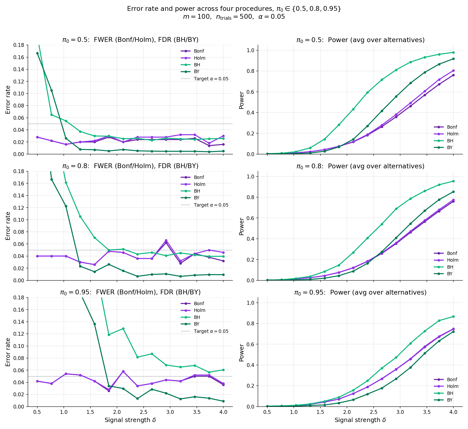
The comparator below runs multiTestingMonteCarlo for a selected procedure across a grid of signal strengths at , . For BH, the FDR curve stays pinned near (below the line) at all , while the FWER curve climbs toward 1 as increases — BH does not control FWER. For Bonferroni / Holm, FWER stays near and FDR slopes down. The power curve in the right panel shows BH’s advantage: at moderate , BH’s power is more than double Bonferroni’s.
Procedure: Benjamini–Hochberg, m = 100, π₀ = 0.80, α = 0.050, 300 MC trials at each of 9 δ grid points. FDR target under independence: α·π₀ = 0.040.
20.7 The Benjamini–Hochberg Procedure
We now prove the featured theorem of Topic 20.
Order the -values ascending: . Let be the largest rank such that (set if no such exists). The Benjamini–Hochberg procedure rejects — i.e., the hypotheses with the smallest -values.
If the -values are independent (or positively regression-dependent on the subset, PRDS), then
Proof Proof 5 — BH FDR control (featured) [show]
The argument decomposes the expected FDP into per-null contributions, each of which can be bounded by using an independence-based lemma. We follow BH 1995 for the outline and cite BEN2001 Lemma 2.1 for the key step.
Step 1 — Write the FDP as a sum. For a specific realization of , let denote the total number of rejections when BH is applied at level (so is the actual number of rejections at level ). Then the false-discovery count at the realized is , where the indicator captures whether null is rejected. Dividing by :
Step 2 — Take expectation; condition on the other -values. Taking on both sides and pulling the sum outside the expectation (linearity):
Here denotes the vector of -values excluding , and both and are written as functions of the full -value vector to emphasize that they depend on via the step-up search.
Step 3 — Apply the BEN2001 Lemma 2.1 independence identity. Under independence of the null -values from the rest, Lemma 2.1 of BEN2001 gives, for each ,
with equality in the continuous independent case. The content of the lemma is that the event and the random denominator are coupled in exactly the way BH’s linear-in- threshold is designed to exploit — each unit increment in brings in more null-rejection mass in the numerator while adding worth of dilution in the denominator, and the two balance. See : §§3–4 for the full conditional-expectation expansion; we use the stated bound as a black box.
Step 4 — Sum over the true nulls. Summing the per-null bound from Step 3 over all :
∎ — using linearity of expectation (Step 1–2) and the BEN2001 Lemma 2.1 independence bound (Step 3); BEN1995 original; BEN2001 for the modern formalization.
The proof’s most striking feature is that BH’s FDR control is exactly , not just . The procedure leaves power on the table when — hence Storey’s adaptive correction in §20.8, which estimates from the data and applies BH at level to recover that slack.
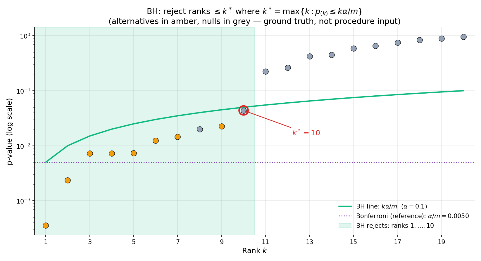
, , . The BH threshold at rank is . Walk from down: , , …, (fail!), (pass — stop). ; reject ranks 1, 2, 3. The critical point: fails its threshold by a hair ( vs ); had it been below, BH would have rejected 4 or more. The regression test T1 in testing.test.ts pins this behavior.
Using multiTestingMonteCarlo('bh', m = 200, π₀ = 0.8, δ = 3.0, α = 0.05, 3000, seed = 123), empirical FDR lands in . The theoretical bound is . Empirical values below are normal — BH is conservative when the signal is strong, because strong alternatives drive up while stays fixed. The test harness T3 in testing.test.ts locks this range. The same simulation shows empirical FWER well above : BH deliberately does not control FWER, and large samples with moderate signal produce many false rejections on their way to producing even more true rejections.
The visualizer below runs the step-up walk one rank at a time. Load the canonical T1 preset, press Step. The active rank descends from , lighting up red (fail) at ranks 10, 9, …, 4, then green (pass) at . The rejection region shades in, containing ranks 1 through 3.
| k | p_(k) | k·α/m | dec. |
|---|---|---|---|
| 10 | 0.5500 | 0.0500 | — |
| 9 | 0.3300 | 0.0450 | — |
| 8 | 0.2100 | 0.0400 | — |
| 7 | 0.0870 | 0.0350 | — |
| 6 | 0.0510 | 0.0300 | — |
| 5 | 0.0430 | 0.0250 | — |
| 4 | 0.0210 | 0.0200 | — |
| 3 | 0.0110 | 0.0150 | — |
| 2 | 0.0030 | 0.0100 | — |
| 1 | 0.0005 | 0.0050 | — |
Regression-test vector from §6.2 T1. BH rejects ranks 1–3 (p_(3) = 0.011 passes threshold 0.015; p_(4) = 0.021 fails 0.020). Expected k* = 3; current k* = 3. The step-up search walks down from k = m, returning the first rank where p_(k) ≤ k·α/m.
The BH threshold function has two endpoints: at (exactly Bonferroni) and at (no adjustment). The linear interpolation between them is what makes the independence cancellation in Proof 5 Step 3 work: the per-rank threshold increment is also the per-rank denominator increment , and the two cancel. Any nonlinear threshold function breaks this. Storey’s adaptive variant (§20.8) rescales to — still linear, but with shrinking the effective .
The BEN2001 Lemma 2.1 independence argument extends to the PRDS (positive regression dependence on the subset) regime — where the conditional distribution of the non-null -values given the null -values is non-decreasing in the null -values. This covers most “positively correlated” scenarios in practice: LD-correlated SNPs in a GWAS, correlated coefficients in a regression with positively-correlated predictors. Under PRDS, BH still controls FDR at . Under negative dependence, BH can fail; §20.8 Thm 6 (BY) handles this case at an power cost.
Unlike Holm, BH is not obtained from closed testing with Bonferroni intersection tests; those would produce Holm. BH corresponds to a different closed-testing construction (Simes intersection tests) that is valid for FWER control only under independence, and the resulting closed procedure controls FDR as well. The cleaner modern view: BH is its own step-up procedure derived directly from the FDR-control calculation of Proof 5, independent of the closed-testing scaffold. Closed testing explains why FWER procedures are nested (Holm dominates Bonferroni); FDR procedures live in a separate algebraic universe.
20.8 Dependence and Adaptivity: BY and Storey
BH under arbitrary dependence (Benjamini–Yekutieli 2001) and BH adaptive to the true null fraction (Storey 2002) are the two major variants practitioners reach for when BH’s assumptions don’t hold or when additional power is available.
Let be the harmonic number. Apply BH with thresholds at rank . Under any joint dependence structure of the -values (positive, negative, or arbitrary), this BY procedure controls FDR at .
The price of universal validity is the factor: , so for the BY thresholds are times smaller than BH’s — a roughly power loss. When independence or PRDS can be reasonably assumed, BH dominates. When dependence is genuinely unknown — rare in practice, but common in theoretical analyses of novel statistics — BY is the safe default. Stated without proof; see : .
Let at a tuning parameter (canonically ). The Storey q-value at rank is
The Storey procedure rejects hypotheses with . Asymptotically (as ), Storey controls FDR at exactly , recovering the -slack that BH leaves on the table.
Storey’s is the fraction of -values above , scaled by to correct for the uniform density. Under the null, ; under alternatives, alternative -values concentrate near zero and contribute little to the above- count. So . Applying BH at — which the q-value construction does — produces tighter thresholds when . Stated without proof; see : . The qvalue Bioconductor package is the de facto bioinformatics implementation.
Simulated hypotheses, 200 true alternatives at effect size , . Bonferroni’s threshold is , so alternatives need -scores above — the tails where only the strongest signals live. BH rejects all -values below at the realized , which for moderate signal lands in the hundreds. The genomics figure below (which will render once the supplementary cell in 20_multiple_testing.ipynb is executed) shows BH recovering roughly more true positives than Bonferroni at the same (empirical) FWER cost.

John Ioannidis’s 2005 paper asked: given a statistically significant finding (), what is the probability the corresponding alternative is true? The answer depends on the prior probability of the alternative. For a screening study with and moderate power : expected true positives ; expected false positives . The positive predictive value . A "" finding in this regime is a false positive of the time. Controlling FDR at aligns the reported significance claim with for the rejected set, which is the practical guarantee that FWER alone does not deliver.
Even researchers who never consciously run multiple tests inflate via unstated analytical flexibility: outcome choice, covariate selection, data cleaning rules, subgroup definitions, alternative models. Each branching analytic decision, if it depends on the data, effectively increases . GEL2014 estimate that a “single” analysis often corresponds to between and latent decisions, so the naive threshold corresponds to an unadjusted FWER of roughly to under the global null. Pre-registration is the technical remedy; multiple-testing correction is the retroactive one.
A/B testing with fixed pre-specified metrics on a common user population: positive regression dependence (PRDS) — BH is appropriate. GWAS within a single chromosome: positive dependence via LD — BH is appropriate. Testing a single hypothesis across many unrelated datasets (pooled meta-analysis with unknown dependence): BY is the safer choice. Post-hoc subgroup analysis with unstated inclusion rules: no procedure saves you — this is the Gelman–Loken regime, and the fix is pre-registration, not a different threshold.
The canonical is a sensible default but not optimal for every distribution. STO2002 proposes a bootstrap-based tuning: compute over a grid and pick the minimizing estimated MSE. For large the choice barely matters; for , the bootstrap can stabilize estimates. The Bioconductor qvalue package runs the bootstrap by default.
If is genuinely close to 1 (GWAS: ), Storey and BH are numerically indistinguishable. The Storey adjustment matters most for moderately dense signals () common in transcriptomics, proteomics, and moderate-dimensional regression coefficient testing. Bioinformatics pipelines default to Storey (via qvalue); statisticians default to plain BH unless they have explicit evidence .
The 2005–2016 replication-crisis literature (Ioannidis, Gelman–Loken, Open Science Collaboration 2015) pointed out that naive in the face of unacknowledged multiplicity produces irreproducible findings at scale. The technical remedy is BH or Storey with appropriately calibrated ; the sociological remedy is pre-registration, adversarial collaboration, and transparency about analytical forking. §17.12 Rem 16 and §17.12 Rem 19-bullet defer to this discussion; both are now fulfilled.
20.9 Simultaneous Confidence Intervals
The test–CI duality of : applies at every level: inverting a level- test gives a CI. Applying the union bound (Bonferroni) or exact formula (Šidák) over parameters produces simultaneous confidence intervals — an -tuple such that
This is the CI-side analog of FWER-controlled testing.
Let be a CI for obtained by inverting a level- test (Topic 19 Thm 1).
(a) Bonferroni simultaneous CIs. Set . Then
(b) Šidák simultaneous CIs. Assume are based on independent test statistics. Set . Then
with equality when every equals the value against which the test was constructed.
Both follow immediately from Topic 19 Thm 1 combined with the union bound (Bonferroni) or the independence product (Šidák). Stated without separate proof.
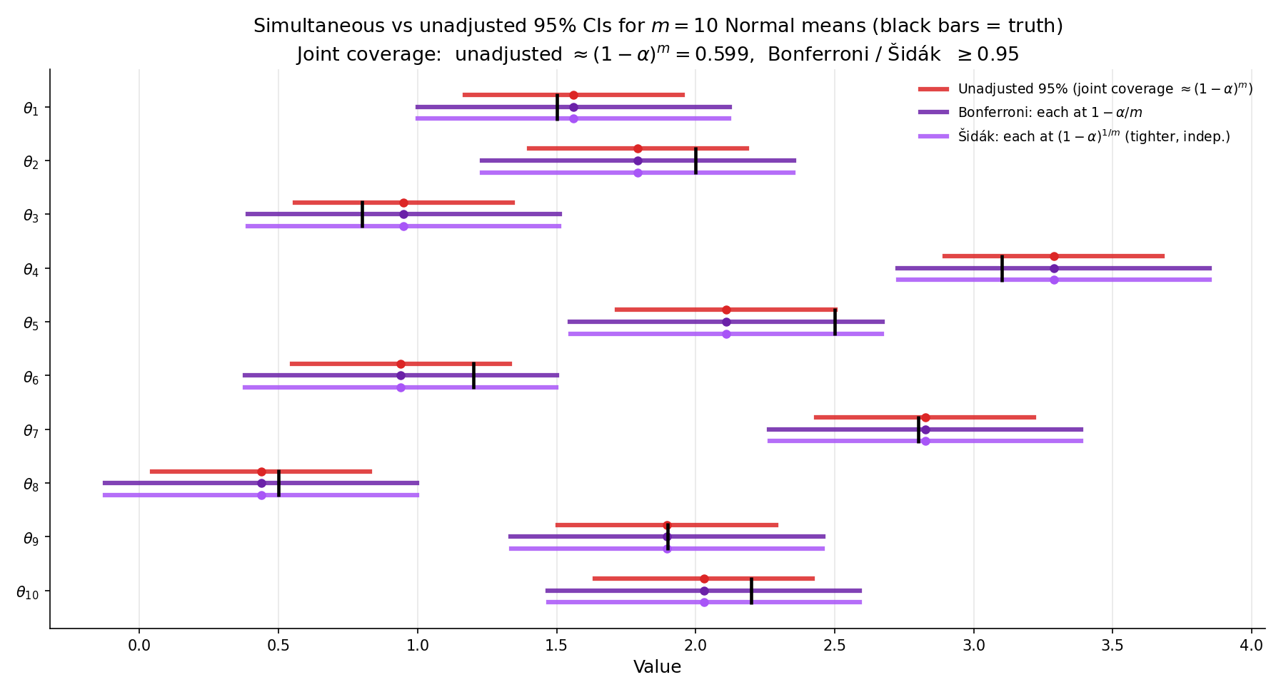
Ten independent sample means with SE , , . The per-interval critical value is , so each Bonferroni CI is . The unadjusted critical value is , giving width . The Bonferroni width is the unadjusted. Over 500 simulations with all true means : empirical joint coverage for unadjusted is ; for Bonferroni .
Same setup as Ex 13. Šidák’s per-interval , so the critical value is — only smaller than Bonferroni’s. CI width is (vs Bonferroni’s ), a gain of . The Šidák construction achieves exact joint coverage under independence, not just , so the marginal gain is worth knowing exists, though the practical difference is negligible.
Matches Figure 8 parameter configuration exactly. Widest Bonferroni CI uses z = 2.807 (vs the unadjusted z = 1.960).
We have covered the general case where no additional structure relates the parameters. Two prominent special cases give tighter bounds:
- Scheffé’s method for linear contrasts in ANOVA: if the parameters of interest are all linear combinations of group means in a one-way ANOVA, Scheffé’s simultaneous CIs use the -distribution critical value, which is tighter than Bonferroni for large . See : or CAS2002 §11.2.4.
- Tukey’s HSD for all pairwise mean differences: exact simultaneous CIs via the studentized range distribution, tighter than Bonferroni when all pairwise contrasts are of interest.
- Working–Hotelling for regression coefficient trajectories: tighter simultaneous bands via the -distribution over a contiguous parameter space.
These are Topic 20’s immediate neighbors and are covered in depth in Track 6’s regression material — §21.8 Rem 16 delivers both Bonferroni-adjusted CIs and Working–Hotelling bands with full F-distribution-based derivations.
An FDR procedure like BH controls the expected false-discovery proportion but does not produce a simultaneous CI — there is no ” joint coverage” interpretation of BH rejections. When the practitioner reports “10 features rejected at BH ,” the claim is that of those 10 are expected to be false rejections, not that the 10 parameters are jointly confined to specific intervals. For joint confidence statements on multiple parameters, Bonferroni / Šidák CIs are the correct tool; for discovery-rate-controlled flag lists, BH is correct.
Topic 19 explicitly deferred simultaneous CIs to Topic 20. The construction above — Bonferroni-adjusted inversion of FWER-controlled tests — is the formal treatment Topic 19 promised. Every claim about test–CI duality in Topic 19 carries over unchanged; the adjustment is to the level (not the construction).
20.10 Track 5 Closes; Multiplicity Lives On
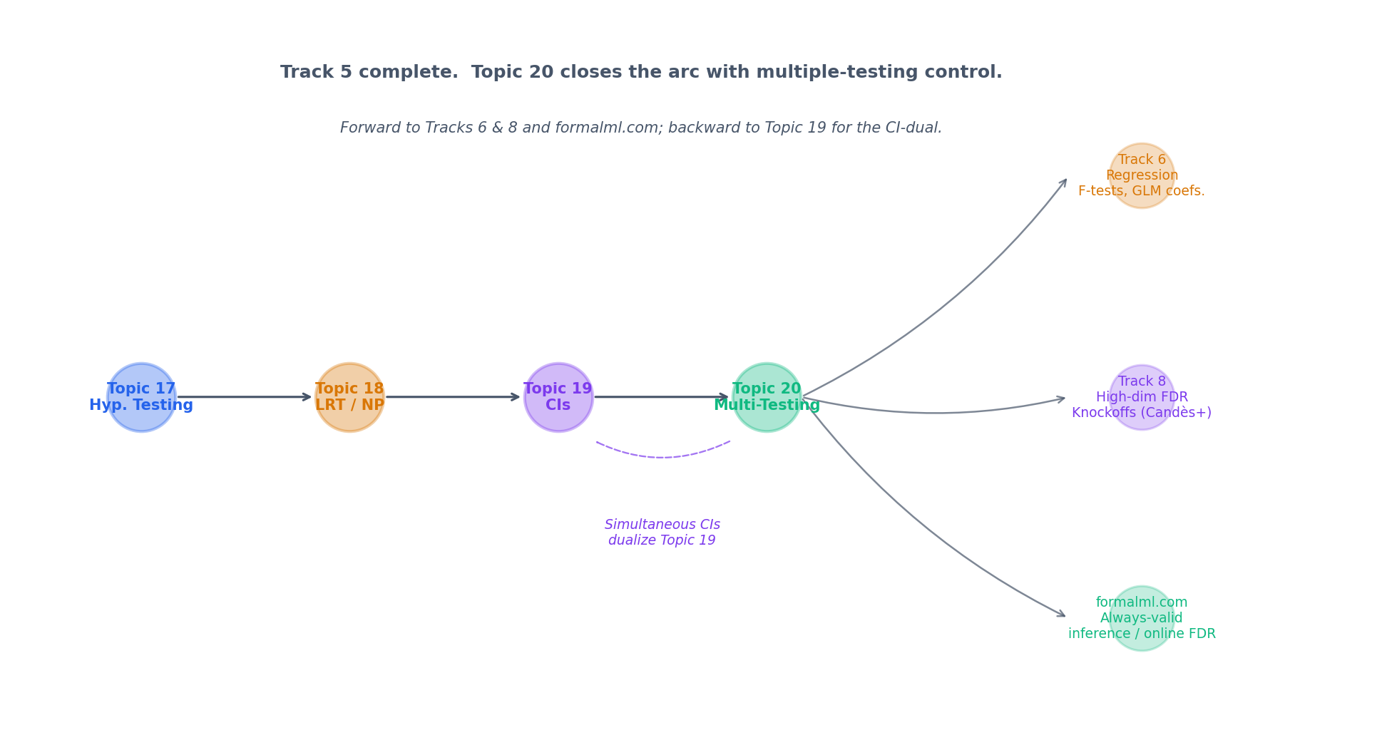
Track 5 — Hypothesis Testing & Confidence — ends here, 4 topics deep. The next tracks inherit this topic’s scaffolding rather than re-derive it:
- Track 6 (Regression) uses Bonferroni-adjusted coefficient CIs (§21.8 Rem 16) as the default simultaneous-inference tool and BH for variable selection. F-tests for nested-model comparisons (§21.8 Thm 9, Example 8) are the closed-testing ancestor of Holm (§20.5 Rem 11).
- Track 7 (Bayesian) contrasts FDR with Bayesian local-FDR (Efron 2010) — the posterior probability that an individual observation is from the null. Bayesian multiplicity reduces to posterior updating; no closed-testing scaffold is required.
- Track 8 (High-Dimensional) builds knockoffs (Barber–Candès 2015) and online FDR (Javanmard–Montanari 2018) directly on top of BH. Every modern multiplicity method traces to §20.7 Thm 5.
The figure below maps Track 5’s arc into these downstream topics.
The setup of §20.3 assumes the hypotheses and stopping rule are fixed in advance. Always-valid confidence sequences (Howard, Ramdas, McAuliffe, Sekhon 2021) and e-processes (Vovk 2019, Grünwald, de Heide, Koolen 2024) dispense with this: the inferential guarantee holds at every stopping time, including data-dependent ones. The mathematical machinery is martingale-based and lives in Track 8 / formalml.com. Every A/B-testing platform that allows “peeking” without Type I inflation uses these tools.
What if hypotheses arrive sequentially and we must decide to reject immediately without seeing future -values? Offline BH no longer applies. The Online-BH procedure (Javanmard–Montanari 2018) and SAFFRON / LORD / Adaptive-LORD family (Ramdas et al. 2018) control FDR in this streaming regime by spending an -wealth budget across time. : lives in Track 8.
Barber–Candès (2015) construct synthetic “knockoff” features exchangeable with the real features under the null, then apply a BH-like step-up on feature-statistic signs. The FDR control at is the §20.7 Thm 5 result extended to a test-statistic-free setting — knockoffs work without requiring the per-feature -values that BH demands. This is the workhorse of modern high-dimensional variable selection.
Westfall–Young (1993) permutation-based multiplicity adjustment computes FWER directly from the joint distribution of the test statistics via resampling, avoiding any dependence assumption. It is the gold standard for FWER control when strict validity is required (e.g., FDA-regulated settings) and computation is affordable. : has the full treatment.
In a fully Bayesian framework, multiplicity is handled by the prior: placing a sparse prior on the -dimensional parameter vector (e.g., spike-and-slab, horseshoe) automatically shrinks most estimates toward zero, achieving a form of implicit multiple-testing correction. The posterior probability that the -th alternative is true is the Bayesian counterpart to the frequentist q-value. Topic 25 §25.10 names this pointer; the full local-FDR framework is developed in Topic 27 §27.9.
We stated Thm 0 (closed testing) without proof in §20.2. The full Marcus–Peritz–Gabriel argument is 15–20 lines and lives in : . The key step is the observation — already stated in §20.2 — that a false rejection requires the true-null intersection’s level- test to reject, which happens with probability .
Hommel (1988) and Rom (1990) are two additional step-up procedures that fall between Hochberg and the full Simes-based closed procedure in the FWER-control hierarchy. Both require independence; both are slightly more powerful than Hochberg on specific -value configurations and slightly less powerful on others. They are named here for completeness; practitioners overwhelmingly default to Hochberg or BH.
References
- Olive Jean Dunn. (1961). Multiple Comparisons Among Means. Journal of the American Statistical Association, 56(293), 52–64.
- Sture Holm. (1979). A Simple Sequentially Rejective Multiple Test Procedure. Scandinavian Journal of Statistics, 6(2), 65–70.
- Zbyněk Šidák. (1967). Rectangular Confidence Regions for the Means of Multivariate Normal Distributions. Journal of the American Statistical Association, 62(318), 626–633.
- Yosef Hochberg. (1988). A Sharper Bonferroni Procedure for Multiple Tests of Significance. Biometrika, 75(4), 800–803.
- Yoav Benjamini and Yosef Hochberg. (1995). Controlling the False Discovery Rate: A Practical and Powerful Approach to Multiple Testing. Journal of the Royal Statistical Society: Series B, 57(1), 289–300.
- Yoav Benjamini and Daniel Yekutieli. (2001). The Control of the False Discovery Rate in Multiple Testing Under Dependency. The Annals of Statistics, 29(4), 1165–1188.
- John D. Storey. (2002). A Direct Approach to False Discovery Rates. Journal of the Royal Statistical Society: Series B, 64(3), 479–498.
- John P. A. Ioannidis. (2005). Why Most Published Research Findings Are False. PLoS Medicine, 2(8), e124.
- Andrew Gelman and Eric Loken. (2014). The Statistical Crisis in Science. American Scientist, 102(6), 460–466.
- Erich L. Lehmann and Joseph P. Romano. (2005). Testing Statistical Hypotheses (3rd ed.). Springer.
- George Casella and Roger L. Berger. (2002). Statistical Inference (2nd ed.). Duxbury.