Bayesian Foundations & Prior Selection
Track 7 opens with the parallel Bayesian formalism: treat θ as a random variable with a prior π(θ), update to a posterior p(θ | y) via Bayes' theorem, and produce every downstream quantity — point estimates, credible intervals, predictions — by integrating against the posterior. The featured result, Bernstein–von Mises, proves that under regularity the posterior concentrates on 𝒩(θ̂_MLE, 𝓘⁻¹/n) in total variation: Bayesian and frequentist inference agree asymptotically.
25.1 Why Bayesian?
Topics 13–24 treated the unknown parameter as a fixed constant: the MLE is a point; confidence intervals are random sets that cover with a specified long-run frequency; hypothesis tests reject or retain fixed null hypotheses. That framework has been extraordinarily productive — every result from point estimation through model selection fits within it — but it answers questions about procedures, not about . A frequentist 95% confidence interval is a guarantee about the interval-constructing procedure, not a probability statement about the parameter.
The Bayesian framework flips the setup. Treat itself as a random variable, specify a prior distribution encoding what we know before observing data, then apply Bayes’ theorem to obtain a posterior distribution that is a probability statement about given the data. Every downstream quantity — point estimates, interval estimates, predictions, model comparisons — follows by integration against the posterior. The price is that we must specify a prior; the return is that every question about admits a direct probability answer.
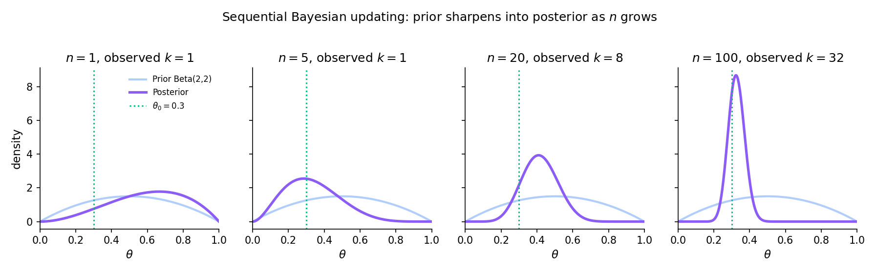
A frequentist answer to “what is ?” is a single number (the MLE) plus an interval around it justified by long-run coverage. A Bayesian answer is a density: the full posterior , which assigns probabilities to every neighborhood of parameter space. Point estimates (posterior mean, posterior median, MAP) and interval estimates (credible intervals, HPD intervals) are summaries of the posterior, not substitutes for it.
The philosophical debate between subjective Bayes (LIN2014 — priors as genuine personal beliefs) and objective Bayes (JEF1961 — priors as reference or non-informative distributions that minimize subjective input) is out of scope for Topic 25. We treat priors as substantive modeling choices whose sensitivity we examine empirically (§25.7), and we note where the two schools diverge as we go.
Topic 25 covers: Bayes’ theorem for (§25.2), Track 7 notation (§25.3), exponential-family conjugacy with full proof (§25.4), five canonical conjugate pairs with Beta-Binomial in full (§25.5), credible intervals and posterior predictive (§25.6), prior selection including Jeffreys (§25.7), Bernstein–von Mises with a sketch proof (§25.8), multivariate Normal-Inverse-Wishart as a pointer (§25.9), and the forward-map to Track 7 (§25.10). It does not cover: MCMC algorithms (Topic 26), Bayes factors or BMA beyond naming (Topic 27), hierarchical and empirical Bayes (Topic 28), variational inference or Bayesian nonparametrics (formalml). Each deferral gets a §25.10 pointer.
25.2 Bayes’ theorem for a parameter
The computational engine is Topic 4 Thm 4 (Bayes’ theorem for events), lifted from a two-event statement to a statement about densities on a continuous parameter space.
Let be an unknown parameter and an observed sample. The Bayesian framework attaches five densities to the inference problem:
- Prior : distribution on encoding information about before observing data.
- Likelihood : the sampling density, viewed as a function of with fixed.
- Posterior : distribution on conditional on the observed data.
- Marginal likelihood : the prior-predictive density of , also called the evidence.
- Posterior predictive : distribution of a future observation integrating out posterior uncertainty.
Under the measure-theoretic conditions of Topic 4 Thm 4 (absolute continuity of the joint distribution with respect to a product measure on ),
where is the marginal likelihood. Equivalently, in unnormalized form,
Proof is a direct application of Topic 4 Thm 4 to the joint density ; the computation is exactly the event version with replaced by density integrals.
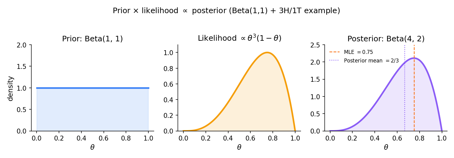
Let and place a uniform prior (flat on ). Observe . Then:
and the unnormalized posterior is
which is the kernel of . Normalizing, , with posterior mean . The data shifted the posterior mean from (prior) to — and shrunk the posterior SD from to .
In practice one rarely computes the marginal likelihood directly — the proportionality together with the constraint determines the posterior uniquely. For conjugate pairs (§25.5) the identification of the posterior kernel with a known density family sidesteps the integral entirely. For non-conjugate cases, MCMC (Topic 26) sidesteps it via ratio-based acceptance.
Posterior Beta(9.0, 15.0). The HPD interval is the shortest 95% credible interval; it coincides with the equal-tailed interval only for symmetric posteriors.
25.3 Track 7 notation conventions
The notation locked in this section propagates to Topics 26, 27, and 28. Every symbol is introduced explicitly; the rationale for the Bernardo–Smith / Robert house style over the Gelman overloading is given below the table.
| Object | Symbol | Interpretation |
|---|---|---|
| Prior density | Distribution over before observing data. Positive, integrable (or improper — §25.7 Def 7). | |
| Posterior density | Distribution over after observing . | |
| Sampling density | or | Likelihood — joint density of given , viewed as a function of . |
| Marginal likelihood | Normalizing constant; also called evidence or prior predictive. | |
| Posterior predictive | Distribution of a future observation integrating out posterior uncertainty. | |
| KL divergence | Relative entropy of w.r.t. . | |
| Bayes factor | Posterior-odds update factor. Topic 25 mentions only; Topic 27 develops. | |
| MAP estimate | Mode of the posterior. | |
| Posterior mean | Bayes estimator under squared-error loss (§25.6 Rem 9). | |
| Posterior median | Bayes estimator under absolute-error loss. | |
| credible set | with | Analog of the frequentist CI in the Bayesian framework. |
| HPD interval | — the set of with | Highest-posterior-density interval — the shortest credible set. |
We use for prior (Bernardo–Smith / Robert house style) because it is visually distinct from the sampling and the posterior — the alternative Gelman-style overloading forces context-based disambiguation in every formula. We write for posterior predictive using tilde-for-new-observation rather than subscripts because tilde renders cleanly in KaTeX. We write for marginal likelihood because the natural alternative collides with the sampling density viewed as a function of . Bayesian and frequentist estimators are distinguished by subscripts throughout: (Topic 14), , , .
25.4 Exponential-family conjugacy
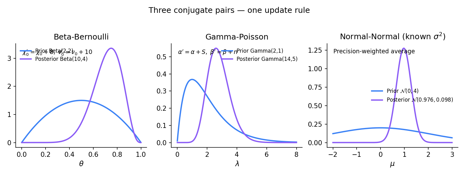
The five conjugate pairs of §25.5 (Beta-Binomial, Normal-Normal, Normal-Normal-IG, Gamma-Poisson, Dirichlet-Multinomial) all emerge from a single construction on exponential families. The theorem below generalizes Topic 7 Thm 3: what was algebra there — close the exponential family under multiplication by a particular kernel — becomes Bayesian inference here, with the updated kernel as the posterior.
A family of distributions is conjugate to a likelihood if, for every prior in the family and every sample , the posterior is also in the family — only the hyperparameters update.
Let be a one-parameter exponential family in canonical form,
with natural parameter , sufficient statistic , base measure , and log-partition . Define the conjugate-prior family indexed by by
where is the normalizing constant (finite whenever the integral on converges). For iid observations with sufficient-statistic total , the posterior is
The hyperparameter is the pseudo-sample-size: the prior is worth equivalent observations before any data arrive. is the pseudo-sufficient-statistic total.
Proof 1 Proof of Thm 2 (exponential-family conjugacy) [show]
Step 1 — setup. Let as stated, with natural parameter and sufficient statistic .
Step 2 — proposed conjugate prior. Define
with hyperparameters , , and normalizing constant chosen so . Whenever this integral is finite, is a proper prior; §25.7 Def 7 handles the improper case.
Step 3 — apply Bayes’ theorem. Given iid observations with joint likelihood
Write for the sufficient-statistic sum. Then, dropping the constant that does not depend on ,
Step 4 — collect exponents. Combining the two exponentials,
Step 5 — identify the posterior kernel. This is the kernel of the same conjugate family with updated hyperparameters , . Since the normalizing constant of the prior family depends only on the kernel shape, we conclude
Step 6 — interpretation of the update rule. The hyperparameter acts as a pseudo-sample-size: the prior is worth equivalent observations before any data arrive. is the pseudo-sufficient-statistic total. After observing real data points with sufficient-statistic sum , the effective sample size grows to and the effective sufficient-statistic total to .
∎ — using Topic 4 Thm 4 (Bayes’ theorem) and Topic 7 §7.7 Thm 3 (exp-family form).
Topic 7 §7.7 Thm 3 constructed the conjugate-prior family for an exponential likelihood — the algebra of Proof 1 Step 4 but stripped of inferential framing. Thm 2 adds the inferential layer: the updated hyperparameters are now the posterior, and every downstream Bayesian quantity (credible interval, posterior mean, posterior predictive) follows from this one identification. Where Topic 7 asked “what family of priors is closed under multiplication by this likelihood?” Topic 25 answers “what is the posterior given this prior and these data?” — but they are literally the same calculation.
The hyperparameter pair is interpretable as a pseudo-dataset of observations whose sufficient-statistic total is . Under this reading, the prior encodes prior information by committing to the equivalent of imaginary observations, and Bayes’ theorem literally concatenates them with the real data. Informative priors have large ; weakly informative priors have ; non-informative improper priors correspond to the formal limit (§25.7). This pseudo-observation framing is the clearest way to calibrate how much prior information to commit.
25.5 The canonical conjugate pairs
Thm 2 is abstract. Making it concrete means specializing to the five canonical conjugate pairs used throughout applied Bayesian statistics. Beta-Binomial is the first and simplest, with a full end-to-end proof. The other four pairs are worked as examples with citation back to the algebra Topic 7 already established.
Let and place a prior on . After observing successes in trials,
The posterior mean is
a convex combination of the prior mean and the sample proportion, with weight proportional to the pseudo-sample-size.
Proof 2 Proof of Thm 3 (Beta-Binomial posterior) [show]
Step 1 — setup. Observe successes in independent Bernoulli() trials; equivalently, observe from . Place a prior on .
Step 2 — likelihood and prior. The Binomial likelihood, viewed as a function of ,
The Beta prior density,
Step 3 — apply Bayes. The posterior is proportional to likelihood × prior:
Step 4 — identify. This is the kernel of . Since the posterior must integrate to 1, the normalizing constant is , and
Step 5 — posterior moments. The posterior mean is
with — a convex combination of the prior mean and the sample proportion , with weights proportional to the pseudo-sample-size and the real sample size .
∎ — using Topic 4 Thm 4 (Bayes’ theorem) and Topic 6 §6.6 Thm 12 (Beta moments).
Let with known, and prior . The posterior on given the sample mean and sample size is with
The posterior precision is the sum of prior precision and data precision — the canonical precision-weighted averaging formula. The posterior mean is the precision-weighted average of the prior mean and the sample mean. Derivation mirrors Proof 2 but with Gaussian kernels; see Topic 7 §7.7 for the exp-family algebra in the location-family case.
When is unknown, place a joint Normal-Inverse-Gamma prior
After observing iid data with sample mean and sample variance , the posterior is Normal-Inverse-Gamma with updated hyperparameters (GEL2013 §3.3 Eqs 3.3–3.5):
The marginal posterior on is a non-standardized Student-t with degrees of freedom, location , and scale — heavier tails than Normal because ‘s uncertainty widens the marginal on .
Let and prior (shape-rate). Observing , the posterior is
with posterior mean . The algebra reduces to the exp-family update rule of Thm 2 with , (Poisson canonical form). See Topic 7 §7.7 Ex 3 for the matching derivation.
Let with , and prior for . Observing counts with , the posterior is
the natural generalization of Beta-Binomial to categories. Topic 8 §8 Thm 6 works this as pure algebra; Topic 25 adds the inferential layer (credible sets on the simplex, marginal posteriors on individual ).
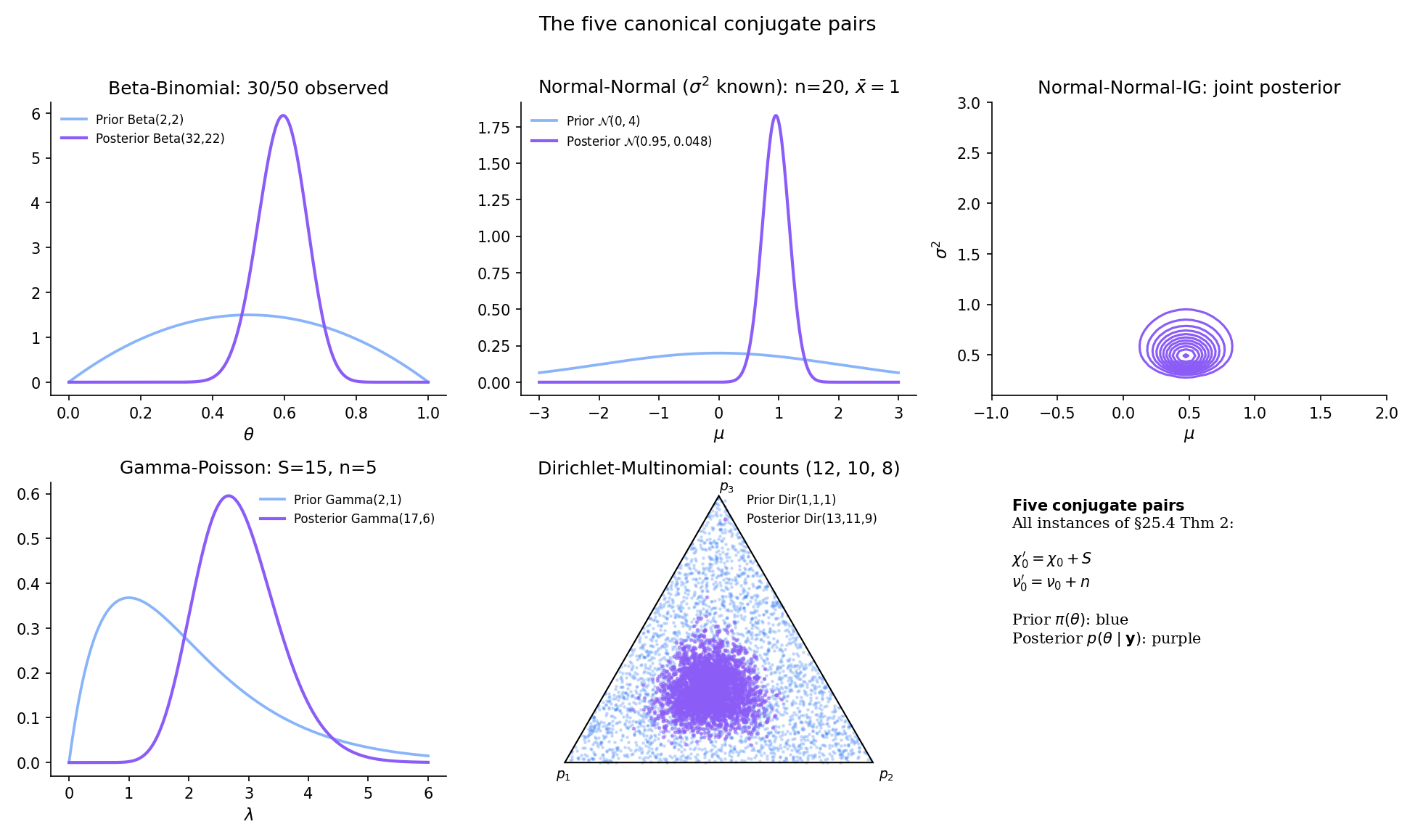
Every pair in §25.5 is a specialization of the exponential-family conjugacy theorem. Beta-Binomial: , (logit-parameterized Bernoulli). Normal-Normal known : , (location-only Gaussian). Gamma-Poisson: , . Dirichlet-Multinomial: the multi-parameter extension where is a count vector. Normal-Normal-IG is the two-parameter case with jointly — the algebra is more involved but the conjugacy logic is identical.
Conjugate priors exist only for exponential-family likelihoods. Non-exponential-family models — mixtures, hierarchical models beyond Topic 28, neural networks — have no closed-form conjugate priors. In these cases, the posterior is known only up to the intractable normalizing constant , and one must resort to approximation: MCMC (Topic 26) for exact asymptotic sampling, variational inference (formalml) for fast approximate posteriors, or Laplace approximation (§25.8 Rem 16) for local Gaussian approximations at the MAP.
Posterior Beta(9.0, 15.0). The HPD interval is the shortest 95% credible interval; it coincides with the equal-tailed interval only for symmetric posteriors.
25.6 Credible intervals and posterior predictive
The posterior is the full Bayesian answer, but practical work demands summaries. Credible intervals are the Bayesian analog of confidence intervals — interval-valued summaries with posterior-probability content. Point estimators (posterior mean, median, MAP) are scalar summaries, each minimizing a different Bayes risk. The posterior predictive closes the loop: given the posterior on , what is the distribution of a future ?
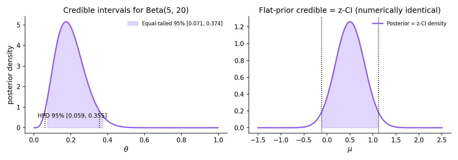
For a posterior and level , a set is a credible set if . Two canonical choices:
- Equal-tailed credible interval: where is the posterior -quantile.
- Highest-posterior-density (HPD) interval: for the largest such that has posterior mass . The HPD is the shortest credible set.
For symmetric unimodal posteriors the two coincide. For skewed posteriors the HPD is narrower and shifted toward the mode.
The three standard Bayesian point estimators of are:
- Posterior mean: .
- Posterior median: , the -quantile of .
- MAP estimate: .
Each is Bayes-optimal under a different loss: posterior mean under squared-error loss, posterior median under absolute-error loss, MAP under 0-1 (indicator) loss — as in .
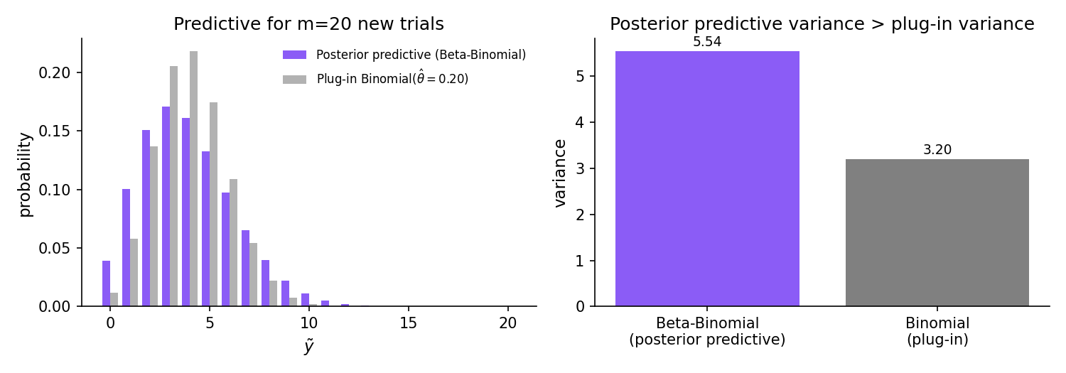
Under the Beta-Binomial setup of Thm 3 with posterior where , , the posterior-predictive distribution of a future count from new independent Bernoulli() trials is the Beta-Binomial compound:
The variance of under the posterior predictive strictly exceeds the variance under the plug-in Binomial — the Bayesian predictive distribution inflates uncertainty to reflect posterior uncertainty in .
Proof 3 Proof of Thm 4 (Beta-Binomial posterior predictive) [show]
Step 1 — setup. Having observed successes in trials with posterior , the posterior predictive is the distribution of a future count from new independent Bernoulli() trials.
Step 2 — definition. The posterior-predictive PMF is the marginal of under the joint distribution , obtained by integrating out :
Step 3 — substitute the likelihood and posterior. With and where , ,
Step 4 — identify the integral as a Beta function. The integrand is the kernel of . Its integral over is , yielding
Step 5 — wider than plug-in. This is the Beta-Binomial compound with parameters . The posterior predictive is wider than the Binomial plug-in approximation, reflecting the posterior uncertainty in — a structural feature of Bayesian prediction that plug-in point-estimate predictions miss. Specifically, by the law of total variance,
where the first term is the average plug-in variance and the second is strictly positive whenever the posterior on has nonzero spread.
∎ — using Topic 4 §4.3 law of total probability and Topic 6 §6.6 Def 3 (Beta function).
Under the standard data scenario used in §25.5 (the posterior hyperparameters from each conjugate-pair example), equal-tailed 95% credible intervals are:
- Beta-Binomial with : (via the Beta-quantile function).
- Normal-Normal with : .
- Gamma-Poisson with : approximately .
- Normal-Normal-IG with df Student-t marginal on : non-symmetric if the df is small.
- Dirichlet-Multinomial on individual : marginal is Beta with hyperparameters .
The HPD interval is slightly narrower and shifted toward the posterior mode in every skewed case (Beta-Binomial for , Gamma-Poisson, asymmetric Dirichlet marginals).
Under squared-error loss , the Bayes estimator — the one minimizing posterior expected loss — is exactly the posterior mean. This is the Bayesian reading of the bias-variance decomposition: the posterior-mean point estimator is optimal in the sense against the posterior, the same way the sample mean is -optimal against the empirical distribution. See ROB2007 §2 for the decision-theoretic development.
For a symmetric unimodal posterior the HPD and equal-tailed intervals coincide. For skewed posteriors (e.g., Beta(2, 20) with pronounced right skew), the equal-tailed interval allocates equal tail mass to each side, including a long right tail of low-density values; the HPD instead follows the density and is strictly narrower. The tradeoff: equal-tailed is invariant under monotone reparameterization; HPD is not.
For Normal-Normal known the posterior predictive for a future is — the posterior variance plus the likelihood variance, again wider than the plug-in . For Normal-Normal-Inverse-Gamma (unknown ), the predictive is a non-standardized Student-t with df — heavier tails still, because ‘s uncertainty further inflates predictive variance. See Topic 6 §6.7 for the Student-t distribution.
25.7 Prior selection
The prior is a modeling choice, not a fact. Every Bayesian analysis commits to some , and different priors yield different posteriors. This section treats prior selection systematically: three classes (informative, weakly informative, non-informative), Jeffreys priors as a reparameterization-invariant reference construction, improper priors and the integrable-posterior condition, and prior sensitivity as an empirical diagnostic.
Priors divide roughly into three informational tiers:
- Informative: encode substantive prior knowledge. Example: a pharmacologist’s prior on a drug’s dose-response parameter based on ten years of related trials. Hyperparameters reflect that knowledge (small posterior variance when knowledge is strong).
- Weakly informative: encode loose, regularization-style constraints. The canonical example is on logistic-regression coefficients (Gelman et al. 2008) — excludes implausible values like without committing to any specific scale.
- Non-informative: minimize prior influence. Jeffreys (§25.7 Thm 5), reference priors (Bernardo 1979 — deferred), flat priors (often improper).
The pragmatic recommendation (GEL2013 Ch. 2): use weakly informative priors by default; use informative priors when genuine prior knowledge exists; use non-informative priors for benchmarking.
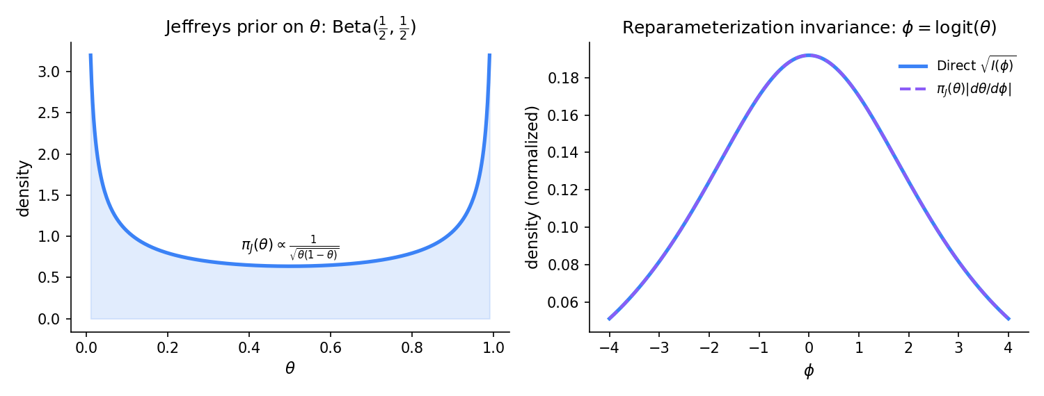
For a one-parameter regular family with Fisher information , the Jeffreys prior is
The Jeffreys prior is reparameterization-invariant: under a smooth monotone reparameterization with Jacobian , — the transformed Jeffreys prior equals the Jeffreys prior computed directly in the -parameterization. This invariance is the principled argument for the Jeffreys construction as a reference prior: any other “non-informative” choice (e.g., const) depends on the parameterization.
Derivation (Bernoulli). For , , so , which is the density up to normalization.
Derivation (Normal-scale). For with known and unknown, , so — the classical log-flat scale prior. (Improper; see Def 7.)
Invariance property proof uses the Jacobian identity for Fisher information: , so . See JEF1961 Ch. III for the full invariance argument.
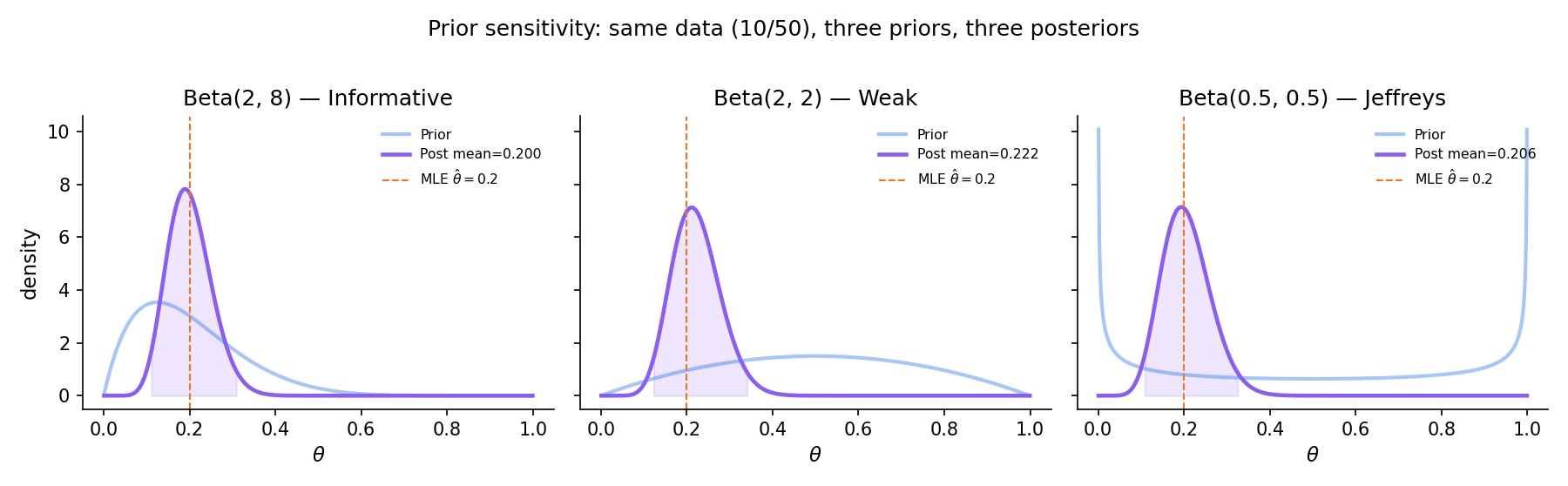
Observe 10 successes in 50 Bernoulli trials. Compare three posteriors:
- Informative peaked at : posterior , mean .
- Weakly informative centered at : posterior , mean .
- Non-informative Jeffreys : posterior , mean .
At all three posterior means lie in — the data dominates the informative prior’s pull toward . At , the three posterior means are far apart (, , ); at they are numerically identical. The interpolation is exactly what Bernstein–von Mises (§25.8) predicts.
CrI = [0.110, 0.309]
CrI = [0.123, 0.341]
CrI = [0.108, 0.326]
Sensitivity magnitude: maxθ |pᵢ(θ | y) − pⱼ(θ | y)| across the three posterior pairs = 2.1054. Slide n to 1000 to watch this decay toward zero — the posteriors align as Bernstein–von Mises kicks in and the prior's contribution becomes negligible.
A prior is improper if — i.e., it is not a valid probability density. Examples: on ; on (the Normal-scale Jeffreys prior).
Bayesian inference with an improper prior is valid if and only if the posterior is proper:
When this integrable-posterior condition holds, the posterior is a well-defined probability density and all downstream quantities (credible intervals, posterior moments, posterior predictive) are well-defined. When it fails, no Bayesian inference is possible.
Improper priors can produce paradoxes when naively combined. Stone (1970) and later Dawid, Stone, and Zidek (1973) showed that two proper-posterior improper priors on nested parameter spaces can yield conditionally inconsistent posteriors — the marginal posterior derived one way disagrees with the marginal posterior derived another way on the same parameter. The resolution requires careful measure-theoretic handling of the improper prior limit. Topic 25 names the paradox once; full treatment deferred to Topic 27 or formalml.
Bernardo (1979) proposed reference priors as a generalization of Jeffreys that maximizes asymptotic expected Kullback–Leibler divergence between prior and posterior — i.e., the prior is chosen to be as “non-informative” as possible in an information-theoretic sense. For one-parameter regular families, reference priors coincide with Jeffreys priors; for multi-parameter problems they differ. Full development is deferred to Topic 27 or formalml.
In applied work, priors are rarely chosen from theoretical principles alone. Prior elicitation — the systematic conversion of expert knowledge into prior hyperparameters — is a substantive modeling activity (ROB2007 §3; GEL2013 §2.9). Practical approaches: ask experts for quantile estimates and fit a prior that matches; use historical data from related problems; elicit pseudo-sample-size directly. The sensitivity analysis of Ex 7 is the diagnostic: if the inference is sensitive to the prior, the prior deserves more attention; if not, the data has spoken.
25.8 Bernstein–von Mises: the bridge to frequentism
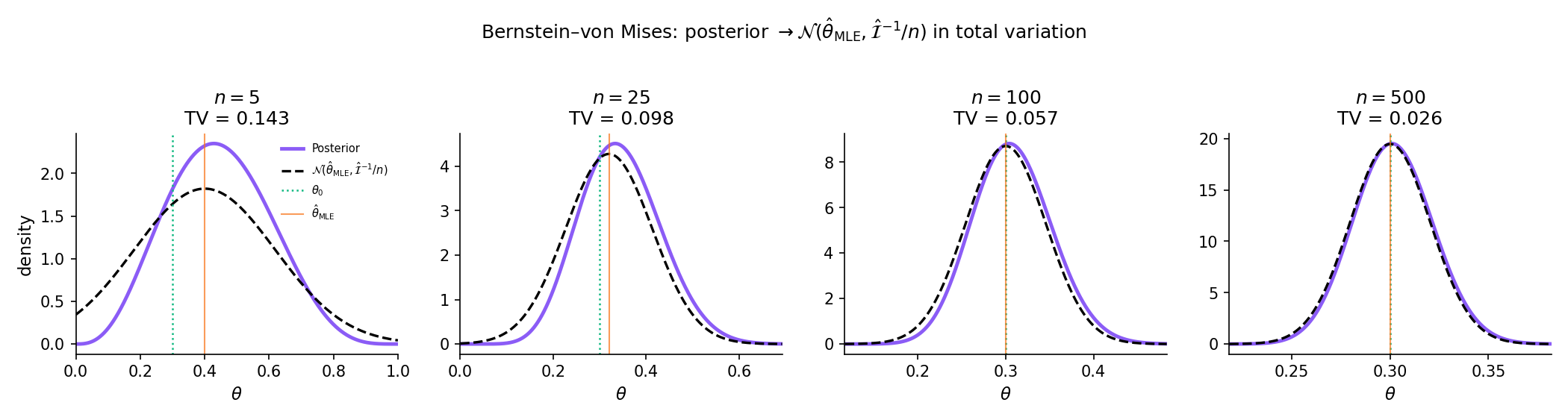
This is the featured section. Under regularity conditions identical to those required for MLE asymptotic normality (Topic 14 Thm 4), the posterior itself is asymptotically Normal — centered at the MLE, with covariance equal to the inverse Fisher information scaled by . Concretely: Bayesian and frequentist inference converge. A 95% credible interval and a 95% Wald confidence interval become numerically identical in the large-sample limit. The prior’s role diminishes at rate ; priors stop mattering once there is enough data.
Let with in the interior of , a regular parametric family with Fisher information . Let be the MLE. For any proper prior continuous and positive at ,
That is, the rescaled posterior converges in total variation to in probability under the true distribution .
Proof 4 Proof of Thm 6 (Bernstein–von Mises, sketch) [show]
Step 1 — statement. As above. We show pointwise convergence of densities then upgrade to total variation via VDV1998 §10.2 Thm 10.1.
Step 2 — Taylor-expand the log-posterior at . Write . The log-posterior is
By Taylor’s theorem, for near ,
for some intermediate . The first-derivative term vanishes because is the MLE (). The second derivative satisfies in probability by Topic 14 Thm 4’s argument.
Step 3 — reparameterize. Let . Then , and
uniformly on compact -sets. This is the Local Asymptotic Normality (LAN) condition; full proof is VDV1998 §7.2 Lemma 7.6.
Step 4 — prior smoothness. Since is continuous and positive at , is bounded on a neighborhood of , and
uniformly on compact -sets (by consistency of , which holds by Topic 14 Thm 3).
Step 5 — assemble the posterior density. In the -parameterization,
This is the kernel of .
Step 6 — extend to total-variation convergence. Step 5 establishes pointwise (at each ) convergence of densities up to normalization. The total-variation upgrade requires showing (a) the posterior puts asymptotically negligible mass outside a shrinking neighborhood of (posterior concentration), and (b) uniform integrability of the posterior density. Both follow from the prior’s positivity at plus the regular-family tail bounds. Full argument: VDV1998 §10.2 Thm 10.1.
Step 7 — interpretation. The posterior forgets the prior at rate : the prior’s contribution to the posterior density becomes vanishingly small relative to the likelihood’s contribution. Bayesian and frequentist inference converge — credible intervals Wald intervals in TV distance.
∎ (sketch) — using Topic 14 §14.5 Thm 4 (MLE asymptotic normality), Topic 11 §11.3 Thm 1 (CLT), and van der Vaart 1998 §10.2 Thm 10.1 (full TV upgrade).
At n=500 the posterior is visually indistinguishable from the Normal-at-MLE.
BvM prediction: as n → ∞, the posterior converges in total variation to N(θ̂_MLE, I(θ₀)⁻¹/n). Watch the purple posterior collapse onto the black dashed Normal curve, and the TV distance drop below 0.01 once n is large enough.
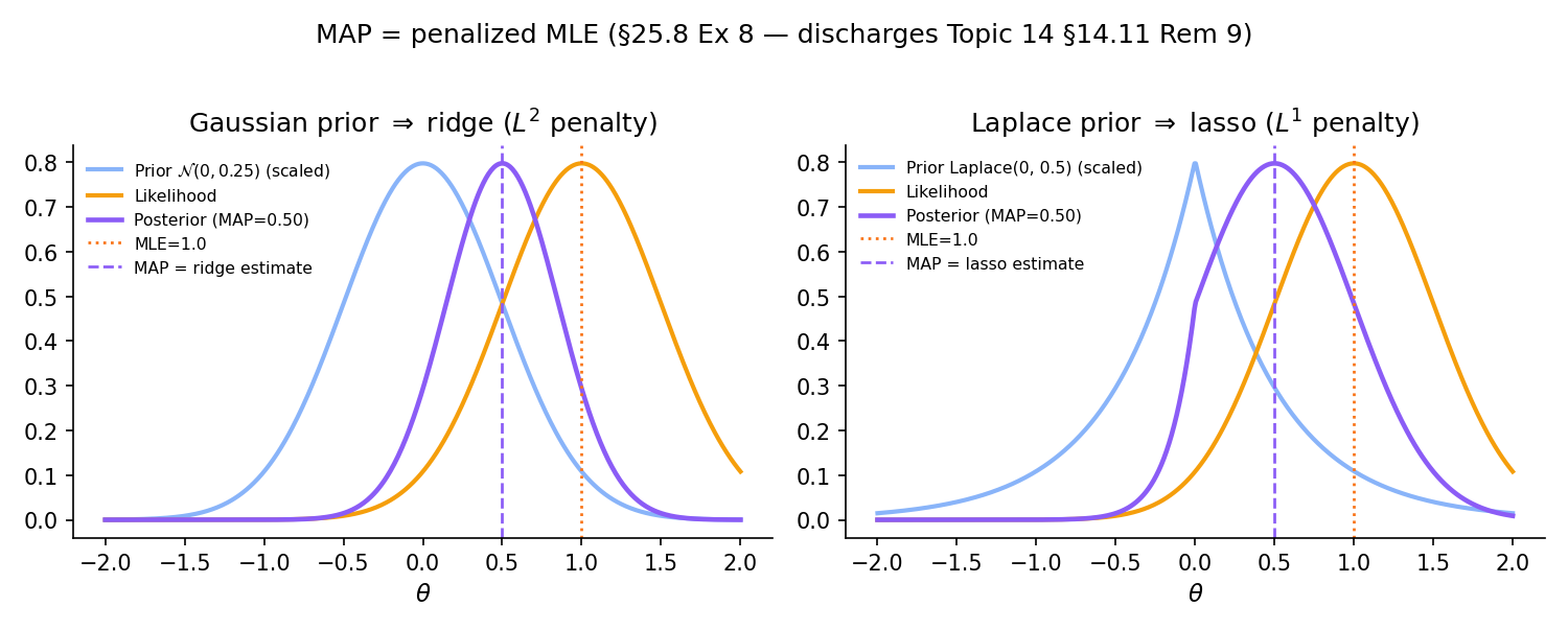
The MAP estimate maximizes the log-posterior:
When is Gaussian, , so maximizes — exactly ridge regression with . When , , so maximizes — exactly lasso with . This discharges Topic 14 §14.11 Rem 9 (the MAP/regularized-MLE correspondence preview) and Topic 23 §23.7 Thm 5 (the MAP-penalization formal correspondence). The arc closes here.
Under BvM, and converge at rate in TV — the regularization vanishes asymptotically, confirming that ridge and lasso are prior-informed procedures whose regularization is a commitment that data eventually overrides.
The same machinery that produces BvM yields a Gaussian approximation to the posterior at any finite — the Laplace approximation. Taylor-expanding to second order at and exponentiating gives where . The same expansion approximates the marginal likelihood:
This is the generalization of Topic 24 §24.4 Proof 2: BIC drops the prior term and approximates , yielding BIC = . The Laplace approximation is the full version — Topic 27 returns to it for Bayes-factor computation.
For the Normal-mean problem with known and improper flat prior , the posterior is exactly — and the 95% credible interval is identical at every finite to the frequentist z-CI. This is not a BvM asymptotic result but a finite-sample coincidence: the flat prior makes the posterior coincide with the sampling distribution of the MLE. This discharges Topic 19 §19.1 Rem 3 and §19.10 Rem 21: for Normal mean under flat prior, Bayesian and frequentist intervals coincide, but the interpretations differ — the Bayesian reads it as “posterior probability that lies in the interval” while the frequentist reads it as “95% of such constructed intervals would cover the true .”
BvM’s regularity conditions are those of MLE asymptotic normality plus positivity and continuity of the prior at . When these fail, BvM can fail:
- Heavy-tailed priors (e.g., Cauchy) violate the -concentration rate near the prior’s tails.
- Non-identifiable models (mixture label-switching, over-parameterized networks) have multimodal posteriors that never collapse to a single Gaussian.
- High-dimensional regimes break the fixed-dimension Taylor expansion of Step 2.
- Nonparametric models (function-valued ) require infinite-dimensional generalizations that sometimes hold (Castillo–Rousseau 2015) and sometimes don’t (DIA1986).
See VDV1998 §10.3 for failure modes in regular models and DIA1986 for the nonparametric counterexamples.
25.9 The multivariate case: Normal-Inverse-Wishart
Topic 25’s scalar framework extends to multivariate parameters. The most-cited multivariate conjugate pair is Normal-Inverse-Wishart — the generalization of Normal-Inverse-Gamma (Ex 3) to joint inference on a mean vector and covariance matrix .
Place a prior — a Normal-Inverse-Wishart distribution. After observing iid Gaussian samples with sample mean and sample scatter matrix , the posterior is NIW with updated hyperparameters. Detailed parameter-update rule: GEL2013 §3.6 Eqs 3.18–3.21. The scalar mechanics of Topic 25 §25.5 Ex 3 (Normal-Normal-IG) are the one-dimensional case.
The NIW framework extends to Bayesian linear regression: place a conjugate Normal-Inverse-Wishart prior on in , and the posterior is NIW with updated parameters that include a ridge-regression posterior mean. Topic 25 §25.5 Ex 3 covered the scalar analog; the full regression generalization, plus non-conjugate priors (horseshoe, spike-and-slab) handled via MCMC, is Topic 27 or Topic 28 territory. This note discharges Topic 21 §21.10 Rem 25.
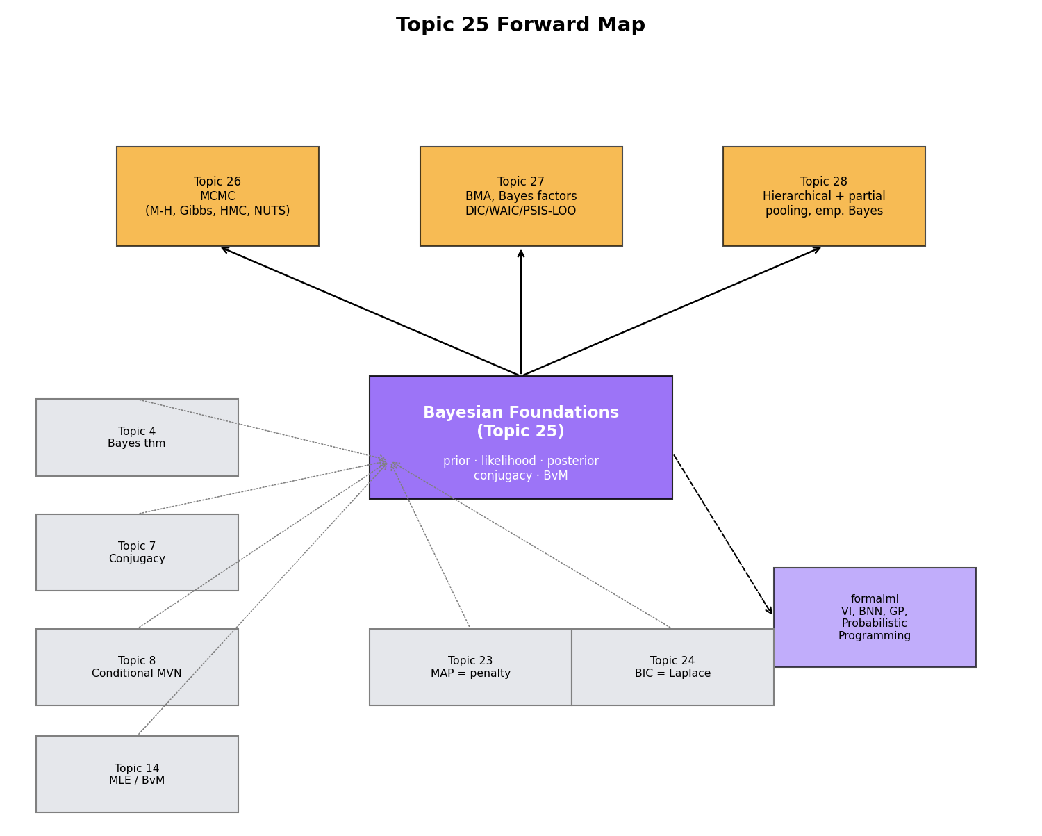
25.10 Forward map
Topic 25 is the Track 7 opener. The remainder of Track 7 — plus one cross-track pointer to formalml — develops the machinery Topic 25 names but defers.
When the conjugate-prior framework fails — non-exponential-family likelihoods, hierarchical models beyond Topic 28, models with many parameters — the posterior is known only up to the intractable normalizing constant . Markov chain Monte Carlo (MCMC) provides exact asymptotic sampling: Metropolis–Hastings (1970), Gibbs sampling (Geman–Geman 1984), Hamiltonian Monte Carlo (Duane et al. 1987; Neal 2011), and the No-U-Turn Sampler (Hoffman–Gelman 2014) are the four principal algorithms. Gibbs samplers use Topic 25 conjugate full-conditionals as building blocks — the connection is direct. Topic 26 develops all four algorithms end-to-end, with the Markov-chain ergodic theorem (§26.7) as the MCMC analog of Topic 10’s SLLN (Thm 10.5).
Bayes factors compare two models via their marginal likelihoods. Bayesian model averaging (BMA) combines posterior predictions across candidate models, weighted by posterior model probabilities. Efficient marginal-likelihood computation uses nested sampling (Skilling 2006), bridge sampling (Meng–Wong 1996), thermodynamic integration, DIC / WAIC / PSIS-LOO (Watanabe 2010; Vehtari–Gelman–Gabry 2017). Topic 25 §25.8 Rem 16 introduced via the Laplace approximation; the full computational machinery is Topic 27. This also houses local-FDR and Bayesian multiplicity (Efron 2010), discharging Topic 20 §20.10.
Topic 25 treats the prior as fixed. Hierarchical priors treat the prior itself as having hyperparameters with their own prior. This is the Bayesian reading of partial pooling (Lindley–Smith 1972): individual-level estimates borrow strength from group-level structure. Empirical Bayes uses the data to estimate directly, collapsing the hierarchy. Continuous shrinkage priors (Carvalho–Polson–Scott 2010 horseshoe) provide adaptive sparsity — the “lasso of priors.” Topic 28 develops.
When conjugate priors break down and MCMC is too slow (hierarchical models with millions of parameters, deep neural networks), variational inference approximates the posterior with a tractable family minimizing . The ELBO (evidence lower bound) machinery, mean-field VI, normalizing flows, and stochastic VI are developed at formalML: Variational Inference .
Every Bayesian point estimator is a Bayes-optimal decision under some loss (§25.6 Rem 9). Bayesian decision theory formalizes this: given a loss , the Bayes decision minimizes posterior expected loss . ROB2007 Ch. 2 is the standard reference; full treatment deferred to a later philosophical essay or formalml.
Bernardo’s 1979 reference-priors framework extends Jeffreys to multi-parameter problems by maximizing asymptotic expected KL divergence between prior and posterior. Intrinsic priors (Berger–Pericchi 1996) generalize improper Jeffreys priors for Bayes-factor computation. These are specialized tools not covered in Topic 25’s introductory opener.
Posterior predictive checks (PPCs) simulate replicated datasets from the posterior predictive and compare them to observed data — a direct Bayesian alternative to frequentist goodness-of-fit tests. GEL2013 Ch. 6 is the standard reference; full development Topic 27.
When the parameter space is infinite-dimensional — distributions over distributions, functions over functions — Bayesian nonparametrics provides the toolkit. Dirichlet processes (Ferguson 1973), Pólya trees, and Gaussian processes as priors are the three principal constructions. GPs were already flagged in Topic 8; full treatment at formalML: Gaussian Processes .
Track 7 is a parallel formalism to Tracks 4–6, not a replacement. Every frequentist method of Topics 13–24 has a Bayesian counterpart: MLE ↔ posterior mean or MAP; Wald CI ↔ credible interval (coincident asymptotically by BvM); LRT ↔ Bayes factor; AIC/BIC ↔ marginal likelihood ; regularization ↔ informative prior. The practical choice between frameworks depends on whether you can defensibly specify priors and whether you want answers that are probability statements about parameters (Bayesian) or long-run frequency guarantees about procedures (frequentist). In many modern applications (hierarchical models, small-sample inference, integration of prior information) the Bayesian framework is better suited; in others (large-n prediction, procedural guarantees with minimal assumptions) the frequentist framework is cleaner. Track 7’s remaining three topics — MCMC, BMA and Bayes factors, hierarchical and empirical Bayes — develop the computational and structural machinery needed to use the Bayesian framework at modern applied scale.
References
- Andrew Gelman, John B. Carlin, Hal S. Stern, David B. Dunson, Aki Vehtari & Donald B. Rubin. (2013). Bayesian Data Analysis (3rd ed.). CRC Press.
- José M. Bernardo & Adrian F. M. Smith. (1994). Bayesian Theory. Wiley.
- Christian P. Robert. (2007). The Bayesian Choice: From Decision-Theoretic Foundations to Computational Implementation (2nd ed.). Springer.
- Harold Jeffreys. (1961). Theory of Probability (3rd ed.). Oxford University Press.
- Dennis V. Lindley. (2014). Understanding Uncertainty (Rev. ed.). Wiley.
- A. W. van der Vaart. (1998). Asymptotic Statistics. Cambridge University Press.
- Persi Diaconis & David Freedman. (1986). On the consistency of Bayes estimates. The Annals of Statistics, 14(1), 1–26.
- George Casella & Roger L. Berger. (2002). Statistical Inference (2nd ed.). Duxbury.
- E. L. Lehmann & George Casella. (1998). Theory of Point Estimation (2nd ed.). Springer.
- Trevor Hastie, Robert Tibshirani & Jerome Friedman. (2009). The Elements of Statistical Learning (2nd ed.). Springer.