Hypothesis Testing Framework
Null, alternative, power, p-values, and the z/t/χ² test family — the decision-theoretic core of classical inference.
17.1 From Estimation to Decisions
Track 4 built the classical estimation toolkit — point estimation, maximum likelihood, method of moments, sufficient statistics, Rao-Blackwell, UMVUE. Track 5 opens a different question. Estimation asks: given the data, what is our best guess for ? Testing asks: is the evidence strong enough to act against the status-quo claim ? The distinction is not cosmetic. Estimation optimizes one quantity (MSE, say); testing trades off two — the risk of rejecting when it is true, and the risk of failing to reject when it is false. This topic builds the framework for that trade-off and applies it to the three canonical parametric families (z, t, ), the binomial exact test, and the asymptotic trio (Wald, score, LRT). Topic 18 extends it with optimality theory (Neyman-Pearson, UMP, Wilks); Topic 19 with confidence intervals via the duality previewed in §17.10; Topic 20 with the multiple-testing correction needed once we admit that a single test rarely stands alone.
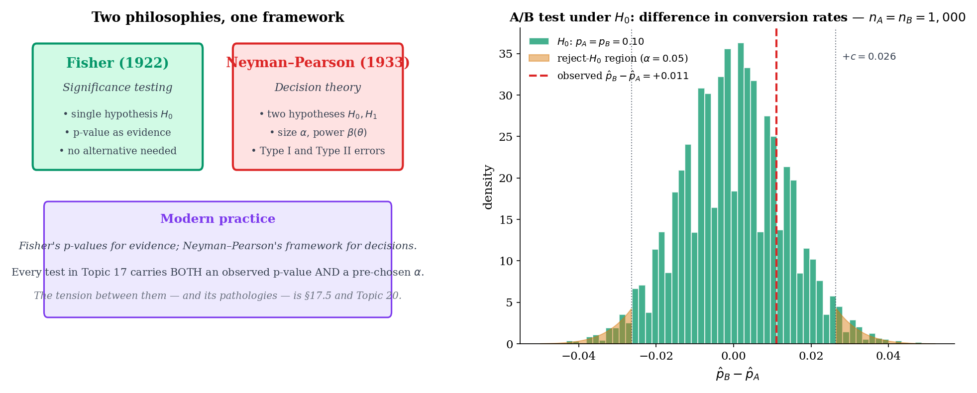
Fisher’s significance testing (1922) framed the p-value as a continuous measure of evidence against a single null hypothesis: small p-values are surprising, large p-values are not, and the analyst uses judgment. Neyman and Pearson’s decision-theoretic formulation (1933) recast testing as a choice between two hypotheses with two error types (Type I and Type II) and two controlled probabilities ( and ). The modern textbook framework merges the two: a test statistic produces a p-value, and the p-value is compared to a pre-specified . Different communities weight the Fisherian and Neyman-Pearsonian views differently, and much of the replication-crisis discourse (Remark 6) stems from confusing the two. Topic 17 develops both threads: §17.5 treats the p-value on Fisher’s terms, while §17.3 and §17.4 set up size and power in the Neyman-Pearson frame.
The running example throughout Topic 17 is the two-variant A/B test. Variant A has conversion rate ; variant B has conversion rate . The question is: does deploying variant B produce a higher conversion rate than the incumbent A? The null is the skeptical baseline (no improvement); the alternative is the claim we might act on. Every experimentation platform — Optimizely, Statsig, internal platforms at Google / Meta / Netflix — runs some flavor of this test billions of times per year. Sample-size calculations (§17.4 Example 6), two-sample proportion z-tests (§17.6 Example 10), and the multiple-testing correction for many simultaneous experiments (§17.11 Remark 16) are the theoretical foundation of that infrastructure. This connects Topic 17 to formalML: A/B testing platforms .
In estimation, we minimize a single risk (mean squared error, say). In testing, we manage two competing risks simultaneously: Type I error (rejecting a true ) and Type II error (failing to reject a false ). These pull in opposite directions — shrinking the rejection region reduces Type I error but increases Type II, and vice versa. No test can drive both to zero at fixed ; the entire Neyman-Pearson framework is built around this trade-off. The pragmatic convention is to fix (Type I rate) at a conventional level (0.05, 0.01, or 0.001) and then maximize power (1 − Type II rate) subject to that constraint. Topic 18 formalizes “maximize power” via the uniformly-most-powerful (UMP) property; here we set up the framework.
17.2 The Hypothesis-Testing Setup
Every hypothesis test is specified by four objects: the two hypotheses, a test statistic, and a rejection region. We formalize the hypotheses first.
Suppose is a sample from a family . A partition with and defines two hypotheses:
- The null hypothesis — the claim we wish to disprove.
- The alternative hypothesis — the claim we wish to act on.
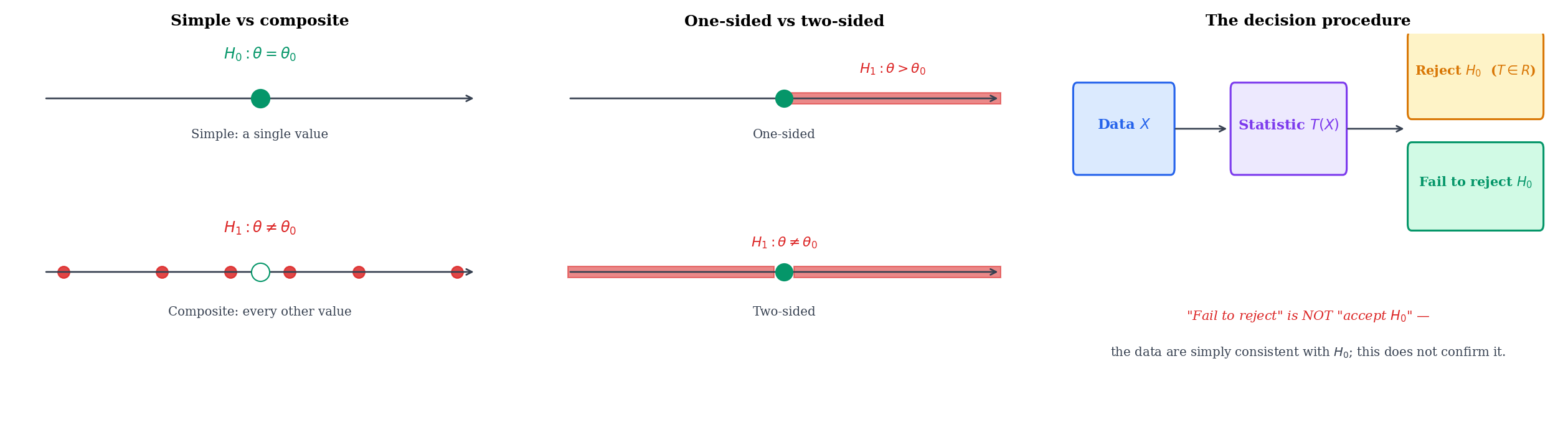
A test is a decision rule that accepts one of or on the basis of the observed data. Note the asymmetry: is the default, retained unless the data provide strong evidence against it. “Failing to reject ” is not the same as “accepting ” — we remain agnostic, having merely failed to accumulate enough contrary evidence.
A hypothesis is simple if is a singleton (one parameter value) and composite otherwise. A test with simple and simple is the cleanest case — Topic 18’s Neyman-Pearson lemma gives a uniformly most powerful test for it. Most real-world tests are composite on at least one side: (simple) vs (composite two-sided) is typical.
For a scalar , the standard alternatives are:
- One-sided right: (used when the analyst has a directional hypothesis — e.g., “the new drug helps”).
- One-sided left: (the mirror image).
- Two-sided: (the agnostic alternative — “something is different”).
One-sided tests are more powerful against alternatives in the specified direction, but they commit the analyst to that direction before seeing the data. Choosing the side after looking at the data is a form of p-hacking (Remark 6).
Variants A and B have conversion rates and . The product team is considering deploying B only if it strictly improves on A. The hypotheses are
Both are composite (each covers an interval in at fixed ). The relevant test statistic (§17.6 Example 10) is the pooled-variance two-sample proportion z-statistic. The one-sided framing captures the business constraint that the team is only interested in improvements, not in detecting arbitrary changes — and, as a bonus, gives more power at fixed than a two-sided test against the same effect size.
If the product team cares whether A and B differ at all — perhaps because a decrease would also prompt action (roll back B; investigate B’s unintended effects) — the two-sided framing is appropriate:
Here is simple (one parameter value: , with forced to equal it) and is composite. The rejection region is the union of two tails, and at the same nominal it has roughly half the power of Example 1 against a given directional effect — the price paid for detecting the opposite direction as well.
A clinical trial compares a new treatment (mean response ) to standard care (). Three framings:
- Simple: , for a pre-specified clinically meaningful effect . Requires knowing up front; rare in practice but crucial for power calculations.
- One-sided composite: , . Matches the regulatory framing: we only approve the treatment if it improves on standard care.
- Two-sided composite: , . Appropriate when an inferior treatment should also prompt action (withdraw, study further).
Choice among the three is a substantive decision driven by the clinical, regulatory, and ethical context — not a statistical one.
17.3 Test Statistics, Rejection Regions, and Size
With the hypotheses fixed, we need a summary of the data that concentrates the evidence for / against , and a rule that uses that summary to make a decision.
A test statistic is a measurable function that maps the data to a single real number. Large (or large for one-sided tests) is interpreted as evidence against ; the reduction is the one we met in Topic 16 under the sufficiency banner, and indeed most canonical test statistics are functions of a sufficient statistic (e.g., the z-statistic is a function of , which is sufficient for in the Normal family with known).
The rejection region is the set of data values for which the test rejects . When is specified via the test statistic as (right-tailed), (left-tailed), or (two-tailed), the threshold is called the critical value and denoted when calibrated to level .
The size of a test with rejection region is
That is, the size is the worst-case Type I error rate over the null set. A test has level if its size is at most — every test of size has level , but a test of level may have strictly smaller size. The distinction matters when the null distribution is discrete (Thm 1, Remark 4, Example 4).
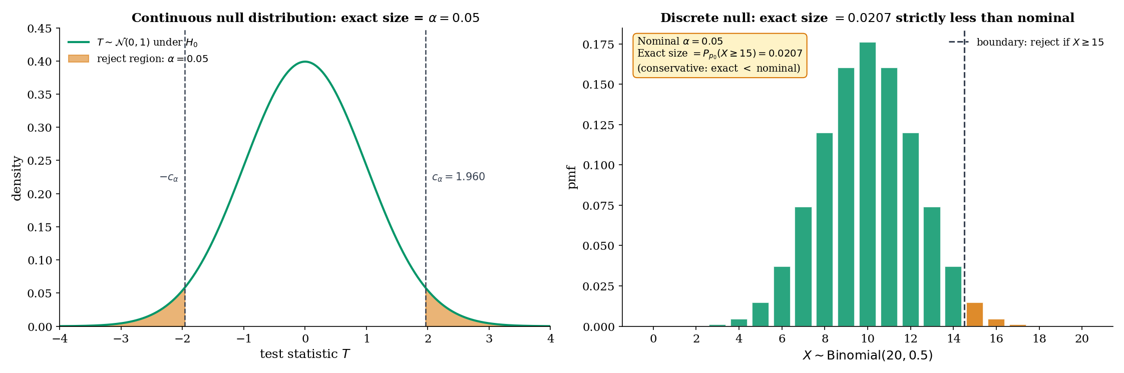
For continuous null distributions, any is achievable exactly: the critical value can be chosen so that on the nose. For discrete null distributions (e.g., Binomial, Poisson), only a countable set of values is achievable; other levels force a conservative test, with actual size strictly less than the designed level.
When the null distribution is discrete, the exact achievable sizes are the tail probabilities of that distribution — a discrete set. For Binomial, the right-tail probabilities at integer give exact sizes — the sizes jump at each integer. A test designed to have level must pick a boundary whose exact size is ; for at , the best achievable right-tailed size is (at boundary ), strictly less than . This is not a flaw; it is the price of exactness. Conservative tests preserve the Type I guarantee at the cost of some power, and they are preferred over alternatives (randomization, mid-p) in most practical settings.
Test vs using with rejection region . Under , , so
The exact size is , so the test is conservative at the nominal . Moving the boundary to would give size — unacceptable. The next smaller achievable size is ; the one after that is . No boundary achieves exactly, and the analyst must choose between conservative () and anti-conservative () rounding. This is the discrete-test pedagogical example that §17.6 Example 11 revisits in the binomial-exact treatment.
17.4 Type I, Type II, and Power
The two errors of a test have names.
- Type I error: rejecting when is true. Its probability is the size (§17.3 Def 6).
- Type II error: failing to reject when is true. Its probability at a specific is conventionally written in the Neyman-Pearson convention where denotes power; some texts reverse this convention and write for the Type II rate. Topic 17 follows Lehmann-Romano: is power (probability of rejection at ), so Type II rate is .
The power function of a test with rejection region is
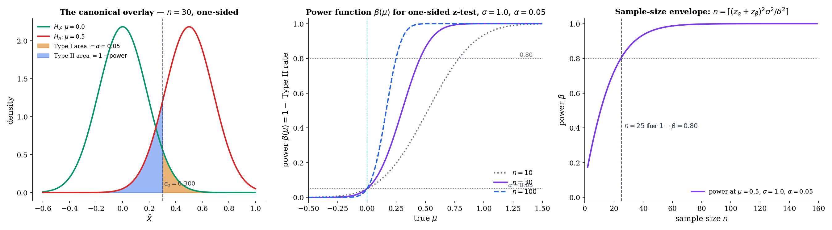
Evaluated at , is the Type I error rate at that null parameter (and , the size). Evaluated at , is the (actual) probability of correctly rejecting at the specific alternative . A good test has close to on and close to 1 on ; how close depends on the sample size and the distance between and .
For a one-parameter exponential family with monotone likelihood ratio (MLR) in the sufficient statistic , the one-sided right-tail test has power that is non-decreasing in . In particular, for any , .
The proof uses the MLR property to show that the likelihood ratio is monotone in , so the event has higher probability at . The full argument uses Topic 18’s optimality machinery; we cite the result here and use it in power calculations that follow.
For iid data with known, consider the right-tailed z-test of vs at level . The test rejects when , where is the -quantile of the standard Normal. Under , , so
This closed-form expression is the analytic engine of the sample-size calculator in Example 6 and the PowerCurveExplorer component. Key observations: increases monotonically in (Thm 2); ; as at rate (the test is consistent).
Suppose we want power against the alternative (a “half-” effect) at level , one-sided. Setting in Example 5 and solving:
Inverting, , so , giving , hence . Rounding up, . More generally, for effect size measured in -units,
the textbook sample-size formula. The PowerCurveExplorer (§17.4 component) implements this closed form for the Normal scenarios and a numerical inversion for the binomial exact test.
In a regular parametric family, the Cramér-Rao lower bound (Thm 13.9) says any unbiased estimator satisfies , where is the Fisher information at . This translates directly into an upper bound on achievable power for any asymptotically-Normal-based test: the smaller the estimator variance, the more concentrated its sampling distribution, and the larger the separation between and sampling distributions — hence higher power. Topic 18 formalizes this as the CRLB giving a “power envelope” that UMP tests achieve. At intermediate level, the intuition is: power is to the estimator’s variance what accuracy is to its bias, and both are bounded below by Fisher information.
β(μ) = 1 − Φ(z_α − √n(μ − μ₀)/σ)17.5 P-values
A rejection region with critical value makes the test a binary decision. A more informative summary — and the one most practitioners actually report — is the p-value.
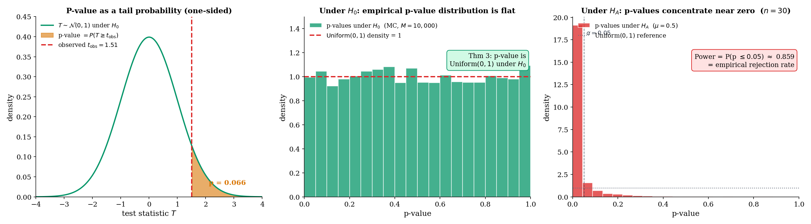
For a test with test statistic and a right-tailed rejection rule , the p-value of an observed data point is
That is, the p-value is the tail probability, under , of the test statistic being at least as extreme as the observed value. For left-tailed tests replace with ; for two-sided tests use for symmetric null distributions (a convention; a few alternatives exist for non-symmetric nulls, discussed in §17.6 Example 11 for the binomial case).
The rejection rule “reject when ” is equivalent to “reject when ” — the two formulations give identical decisions. The advantage of the p-value is that it makes the level at which rejection occurs transparent, rather than forcing an all-or-nothing decision at a fixed .
Let be a test statistic with continuous CDF under . For a right-tailed test, the p-value . Under , .
Proof [show]
Step 1 — identify the distribution of . Under , has CDF . The probability integral transform (Topic 6 §6.3) says that for any continuous CDF and any random variable with CDF , the variable is Uniform. We verify this directly: for any ,
where the second equality uses strict monotonicity of on its support (which holds because is continuous and has full support on that region).
Step 2 — conclude for the p-value. The p-value is . By Step 1, is Uniform under , hence is also Uniform: the reflection is a measure-preserving transformation of , so it maps the uniform distribution to itself.
Step 3 — size calibration. It follows that for every ,
Rejecting when therefore gives a test of exactly size — an appealing formal property of the p-value rule.
∎ — by the probability integral transform (Topic 6) and measure-preservation of on .
Simulate 10,000 samples of size from (the null distribution). For each, compute the z-test statistic and its right-tailed p-value . The histogram of the 10,000 p-values is visibly flat on — the empirical verification of Thm 3. Under an alternative (say ), the same MC run gives a histogram concentrated near zero: power visualized as a distribution on the p-value scale. The PValueDemonstrator component (§17.5) makes this interactive.
A string of papers from the 2005–2016 period argued that naive p-value interpretation is a major driver of non-replicable research. Ioannidis (2005), Why Most Published Research Findings Are False, used a prior-probability argument to show that a statistically significant finding () is often more likely to be a false positive than a true positive, depending on the prior probability of the null — p-values are emphatically not . Gelman & Loken (2013), The Garden of Forking Paths, argued that even well-intentioned researchers inflate Type I error through researcher degrees of freedom (p-hacking, HARKing) without formal multiple testing. The ASA Statement on p-Values (Wasserstein & Lazar, 2016) synthesized the critique into six principles, emphasizing that a p-value quantifies inconsistency with a null model under specific assumptions, not the probability of a hypothesis, and not the importance of an effect.
These are genuine warnings; Topic 20 addresses the multiple-testing piece formally (Bonferroni, Holm, Benjamini-Hochberg FDR, Šidák — see especially §20.7 for the featured BH proof and §20.8 for the Ioannidis / Gelman-Loken framing). For Topic 17, the takeaway is: a p-value is a single number reporting a tail probability under a stated null; it is not a posterior probability, not an effect size, and not a replacement for thinking about the experimental design, power, and prior plausibility.
17.6 The z-test
The z-test is the simplest test in the parametric toolkit: standardize the sample mean, compare to a standard Normal quantile. It is the direct consumer of the Central Limit Theorem (Topic 11 Thm 11.1) and the prototype for every asymptotic test in §17.9.
One-sample z-test. For iid data from a distribution with mean and known variance , the z-statistic for testing is
Under , and under Normality of the data, exactly. For non-Normal data, under by the CLT — an asymptotic result with finite-sample accuracy governed by Berry-Esseen (Topic 11 §11.4).
Two-sample z-test. For two independent samples and with known variances and , the two-sample z-statistic for testing is
Under (and Normality or asymptotically), .
Let be iid with known. For the two-sided test that rejects when (where and ), the size is exactly .
Proof [show]
Step 1 — null distribution of . Under , the sample mean exactly — Normal-sum closure (Topic 6 §6.5) says a sum of iid Normals is Normal with the expected mean and variance. Standardizing,
exactly — no asymptotics needed.
Step 2 — compute the size. The size is . Split into two tails:
By symmetry of the standard Normal density around zero, . And by definition of ,
Adding the two tails,
Step 3 — asymptotic extension when is estimated. If is unknown and replaced by a consistent estimator (e.g., the sample variance), the ratio has null distribution only asymptotically — by the CLT applied to and Slutsky’s theorem (Topic 9) applied to the ratio . Exact size is only in the -known case; for the -unknown case, the t-test (Thm 5) gives exact finite-sample size.
∎ — using Normality of sums (Topic 6), symmetry of the standard Normal, and Slutsky’s theorem (Topic 9) for the asymptotic case.
A random sample of adults has mean IQ and we wish to test whether the population mean differs from the standardized value , assuming (the calibration target of the instrument). The z-statistic is
Two-sided p-value: . At we fail to reject. The point estimate is higher than , but the evidence is not strong — a half- effect would need to reach power 0.8 (Example 6), and we observed about .
A trial enrolls patients in the treatment arm (blood-pressure reduction mmHg, assumed ) and in the placebo arm (, ). Testing :
Two-sided p-value — strongly significant. The observed treatment effect of mmHg at these standard errors is well outside the rejection region at any conventional .
An experiment ran impressions per variant. Variant A produced conversions (); variant B produced (). Testing with the pooled-variance z-statistic:
Two-sided p-value ; we fail to reject at . The detected lift (0.6 percentage points, 5% relative) is plausible — but not strong enough at this sample size. A typical platform would either run the experiment longer or accept the null (“no detectable effect”) given the sample-size budget. This is the canonical output of every A/B-testing platform on the planet; the interactive version of this calculation is in the NullAlternativeSimulator and PowerCurveExplorer components.
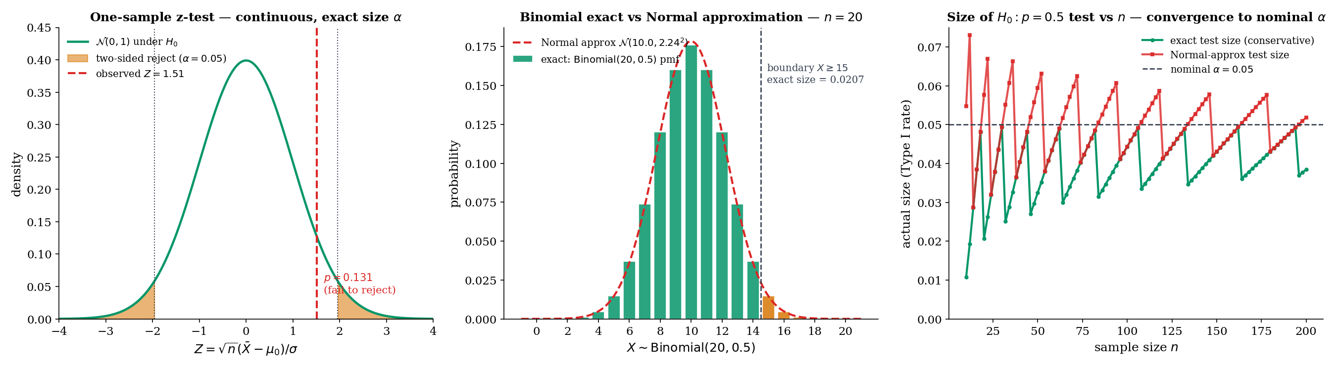
Return to vs at with observed . Two approaches:
Exact test. The null distribution of is . The right-tailed p-value is the exact tail probability:
At , we reject. The rejection region has exact size — conservative (Remark 4).
Normal approximation. Under , ; the standardized observed value is , giving p-value . With a continuity correction (using instead of ), the p-value becomes — close to the exact. Without continuity correction, the Normal approximation overstates significance.
Why this matters. At , the Normal approximation p-value can be 30-40% off the exact p-value at moderate thresholds. At it is typically within a few percent. The notebook figure (right panel) shows the size comparison across : exact size stays below by a discrete jump; Normal-approximation size oscillates above and below , converging as . The binomial exact test has the additional property — covered in Topic 18 — of being UMP one-sided for the Bernoulli family.
For small- discrete tests, the Normal approximation can miss the actual size by several percentage points — not an academic concern but a practical one. An experimenter who believes their nominal is but whose actual Type I rate is is reporting misleading guarantees. For A/B tests at in the hundreds or more, the Normal approximation is typically accurate to within a percentage point; for medical or behavioral studies at , exact tests are the responsible choice. The PowerCurveExplorer component includes a Binomial exact scenario that inverts the exact size via root-find (not the Normal approximation), letting the reader see this effect directly.
17.7 The t-test via Basu
The one-sample t-test is the small-sample analog of the z-test: use (the sample standard deviation) in place of when is unknown. The substitution is natural, but it has a non-obvious consequence: the test statistic no longer has a Normal null distribution. Under iid Normal data, it has a Student’s distribution, and the derivation of that fact is the content of this section. The hinge is Basu’s theorem (Topic 16 §16.9) — the single most important cross-reference from Track 4 into Track 5.
One-sample t-test. For iid Normal data with both and unknown, the t-statistic for testing is
Under , (Student’s t distribution with degrees of freedom) exactly — Thm 5 below, via Basu.
Two-sample pooled t-test. For two independent iid Normal samples with a common unknown variance, the pooled t-statistic for testing is
Under and the common-variance assumption, exactly. When variances are unequal, Welch’s modification (welchTStatistic in testing.ts) gives an approximate distribution with Satterthwaite degrees of freedom — asymptotic exactness only.
Let be iid with both parameters unknown. Under , the one-sample t-statistic
has distribution exactly.
Proof [show]
Step 1 — build Student’s from its defining ratio. The distribution is defined (Topic 6 §6.6) as the law of
where , , and . We will rewrite in this form and verify the three conditions.
Step 2 — express as a ratio of standardized quantities. Under ,
The numerator is under (Topic 6 Normal-sum closure; same as in the z-test’s Proof 2 Step 1). Call it .
Step 3 — identify the chi-squared denominator. The scaled sample variance is
It is a classical result (Topic 6 §6.6; proved via the orthogonal transformation argument in Casella-Berger Thm 5.3.1) that under iid Normal data,
Call this random variable . Then , and
This matches the defining ratio for Student’s — provided .
Step 4 — independence via Basu. This is the hinge. For iid data at fixed , is complete sufficient for — a standard application of the exponential-family completeness result (Topic 16 §16.6 Lemma 1 specialized to the one-parameter Normal with known). The sample variance is ancillary for — its distribution depends on but not on , because is a function of the centered data which is location-invariant. By Basu’s theorem (Topic 16 Thm 7),
Continuous functions of independent random variables are independent, so
i.e., .
Step 5 — conclude. The ratio has , , and — exactly the defining conditions for . Hence under .
∎ — using Normality of (Topic 6), the result (Topic 6 §6.6 / Casella-Berger 5.3.1), and Basu’s theorem (Topic 16 Thm 7 §16.9).
A small clinical study measures fasting glucose in patients on a new regimen: mg/dL, mg/dL. Testing (the standard reference value) two-sided:
Using t: Two-sided p-value from the distribution: .
Using z (wrong!): Two-sided z-approximation p-value: .
The t p-value is larger than the z approximation — the density has heavier tails than , so extreme values are less surprising under and the resulting p-value is larger. For small , ignoring this difference inflates the Type I rate. At the discrepancy shrinks to ; at it is negligible.
A lab tests two catalysts for a reaction yield: trials with catalyst A (, ), trials with catalyst B (, ). Testing with equal-variance pooling:
Two-sided p-value from : . We fail to reject at ; the observed difference in yields is consistent with sampling noise at this . For a detectable effect at with , a similar magnitude would need roughly per arm — a typical power-calculation output.
Proof 3 Step 4 is the load-bearing step. Without Basu’s , the ratio has a distribution that depends in a complicated way on the joint distribution of — and is no longer the answer. Every finite-sample inference procedure for the one-sample Normal mean with unknown variance — the t-test, the t-confidence-interval, and their two-sample siblings — rests on this independence. Topic 16 gave Basu with a full proof and flagged the forward payoff; Topic 17 §17.7 is that payoff. For the featured visualization of this, see the TTestBasuFoundation component below, which shows the decorrelated scatter of across MC replications, the resulting t-statistic histogram matching , and a direct link back to Topic 16 §16.9.
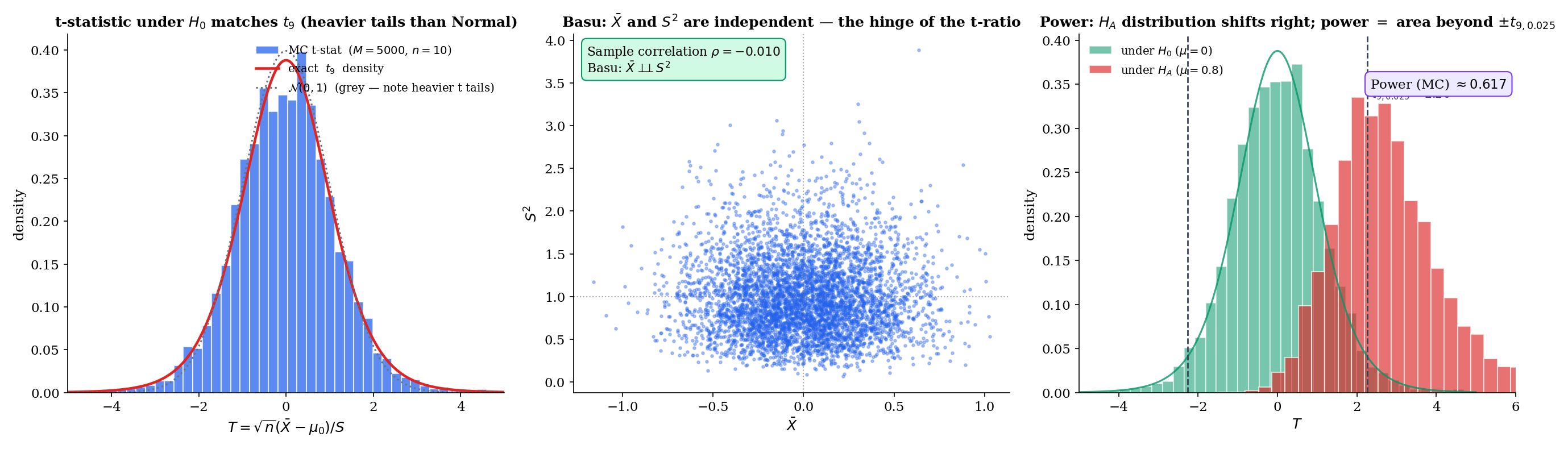
Basu's theorem (Topic 16 §16.9) gives X̄ ⊥⊥ S². This independence is what makes the t-ratio have a clean distribution:
- Numerator √n(X̄ − μ₀)/σ ~ N(0, 1)
- Denominator S/σ = √(χ²_9/(n − 1))
- And they are independent.
That's exactly the defining construction of Student's t_9. Without Basu's independence, the ratio has a messy joint distribution that depends on (μ, σ²).
→ Jump to §16.917.8 The χ²-test
Variance inference and goodness-of-fit are the two classical uses of the chi-squared test. The first tests directly; the second tests whether observed category counts match expected counts under a hypothesized multinomial model (Pearson’s original formulation, 1900).
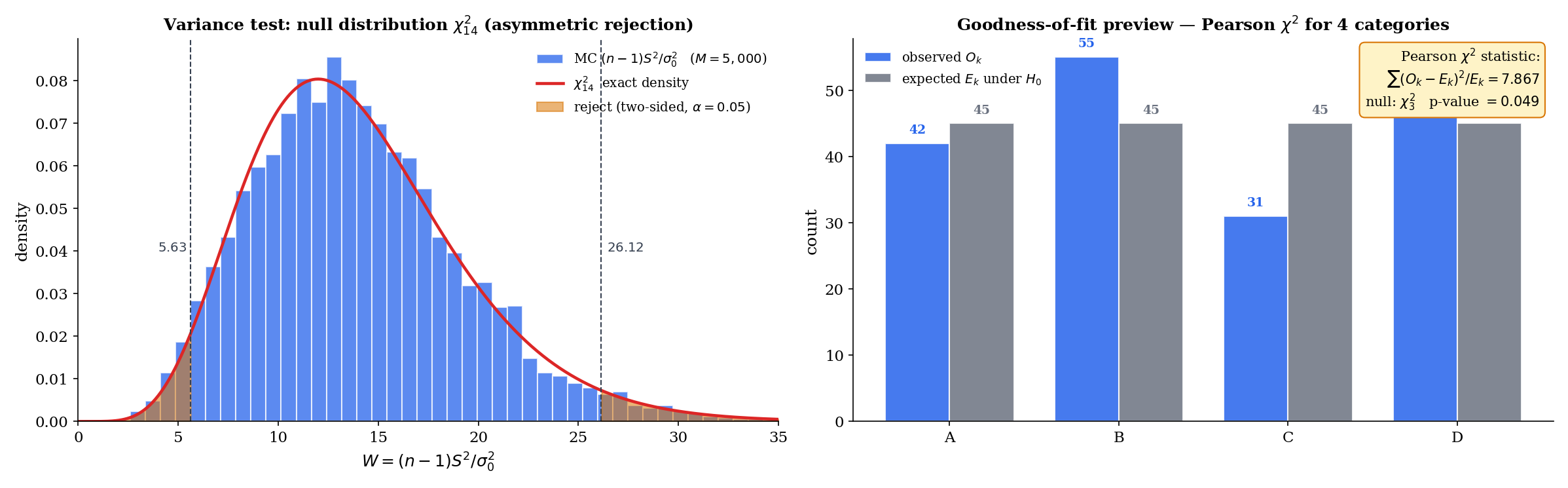
Variance test. For iid Normal data with unknown , the test statistic for is
Under , exactly (Thm 6 below).
Pearson goodness-of-fit. For a categorical distribution with cells, observed counts (summing to ), and expected counts under , the Pearson statistic is
Under , and assuming all are not too small (rule of thumb: ), where is the number of parameters estimated from the data (zero if the null fixes all cell probabilities). The derivation is asymptotic, based on the multinomial CLT and continuous mapping.
For iid data under , the test statistic has distribution exactly.
Proof [show]
Step 1 — reduce to the standard-Normal form. By definition,
Let ; under , iid. Then , so
The problem is reduced to: what is the distribution of when the are iid standard Normal?
Step 2 — orthogonal decomposition of the sum of squares. Expand and collect:
The middle sum is zero because identically. So
Step 3 — distribute the chi-squared degrees of freedom. The left side: because iid (Topic 6 §6.6, sum of squares of iid standard Normals). The last term on the right: , and under iid standard-Normal data, so .
Step 4 — independence + MGF additivity give the split. By Basu’s theorem (as in Proof 3 Step 4), . Hence the decomposition
writes a variable as the sum of two independent non-negative random variables, one of which () is . By the additivity of independent chi-squared variables (Topic 6 §6.6 via the MGF argument: the MGF is , so products of MGFs sum the degrees of freedom), the other term must be :
∎ — using the representation of (Topic 6), Basu’s independence (Topic 16 Thm 7), and MGF additivity for independent chi-squareds.
A manufacturing process specifies (mm²) for a critical dimension. A sample of units has . Testing vs (right-tailed, since excess variance is the quality concern):
Right-tailed p-value from : . We reject at (narrowly) — evidence that the process variance exceeds the specification. Contrast with the two-sided version: for a two-sided variance test at , we use the equal-tailed p-value — we would not reject. The asymmetry of the density makes the two-sided variance test less powerful than the one-sided version against one-sided alternatives.
A die is rolled times; the six face counts are . Under : the die is fair ( for all ):
Right-tailed p-value from (df , no parameters estimated): . The observed counts are easily consistent with a fair die. Note that the asymptotic here rests on the multinomial CLT, and degrades when some are small ( is the classical rule of thumb); Lehmann-Romano Ch. 14 covers small- corrections.
For two independent iid Normal samples with possibly different variances, the ratio has an null distribution under . This is the F-test for equality of variances, and it is the direct generalization of the one-sample variance test to two samples. The F-test also underlies the analysis of variance (ANOVA) and the regression -test for joint significance of coefficients. The full treatment belongs to Linear Regression (Track 6), where the Normal linear model gives the F-test its natural home — see §21.8 Thm 9 (F-test-as-Wilks) and Example 9 (one-way ANOVA).
17.9 Asymptotic Tests: Wald, Score, LRT
The z-test, t-test, and -test all rely on special distributional assumptions (Normality and known families) to give exact null distributions. For general parametric models, three asymptotic tests built directly from the likelihood are the workhorses. They agree to first order under and diverge in finite-sample power — a divergence that Topic 18 §18.8 treats in full.
For a scalar parameter with MLE and Fisher information (Topic 13 Def 13.6), the Wald test statistic for is
Intuition: is the squared standardized distance of the MLE from the null, scaled by the observed information. Under and standard regularity conditions, .
For vector-valued , the Wald statistic generalizes to , asymptotically .
For the same setup, the score test (also called the Rao or Lagrange-multiplier test) uses the score function evaluated at the null:
Under and regularity, . The score test has the desirable property that it only requires fitting the null model (no unrestricted MLE is needed) — a practical advantage in GLM and logistic regression applications where the null fit is much easier than the full fit.
The likelihood-ratio statistic is
It is the log-likelihood difference between the restricted fit (at ) and the unrestricted fit (at the MLE ). Under and Wilks’ regularity conditions, where is the number of restricted parameters (Wilks 1938; full proof in Topic 18).
Under standard regularity conditions (the MLE is consistent and asymptotically Normal per Topic 14 Thm 14.3; the Fisher information is continuous and positive at ; the log-likelihood is sufficiently smooth), the three statistics all have asymptotic null distribution :
The Wald case follows inline from Topic 14 Thm 14.3 (MLE asymptotic normality) by Slutsky and continuous mapping — derived below. The score and LRT cases are stated; Wilks’ full proof of the LRT case is Topic 18’s territory.
Derivation of the Wald case (inline). By Topic 14 Thm 14.3, under ,
Therefore
By consistency of and continuity of , , so . By Slutsky,
Squaring and applying the continuous mapping theorem (Topic 9):
This two-line argument from Topic 14 is all that’s needed for the Wald case. The score case uses a similar argument applied to the score function (one Taylor expansion at ); the LRT case (Wilks) requires a more delicate quadratic-approximation argument that Topic 18 develops in full.
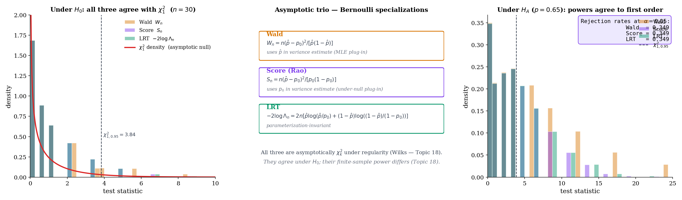
Let iid Bernoulli, . For :
Wald:
Variance estimate at the MLE: .
Score:
Variance estimate at the null: .
LRT:
Under , all three are asymptotically (Wilks, Wald, Rao). The three statistics differ by the choice of variance estimate (Wald uses , score uses , LRT uses an information-theoretic hybrid via the KL divergence). At and , MC simulation under (5000 replications, testing.ts test #17) confirms all three have empirical mean and empirical quantiles matching .
A short Taylor expansion of the log-likelihood around reveals that all three statistics are asymptotically equivalent under :
At finite they differ, and the differences matter for power at alternatives close to the null; they can also matter for finite-sample Type I error in small samples. Topic 18 treats the finite-sample divergence quantitatively.
One practical advantage of the LRT is that it is invariant under reparameterization. If we replace with (any smooth one-to-one transformation), the log-likelihood ratio is unchanged — the maximized likelihoods are the same, just at different parameter values. Hence the LRT statistic and its p-value are identical under reparameterization.
The Wald statistic, by contrast, is not invariant: and can differ substantially when is nonlinear — and their asymptotic distribution is only approximately right at either end. This is a common source of confusion in practice; for logistic regression (natural parameter vs original parameter ), Wald statistics on and on can give meaningfully different p-values. Practitioners often prefer the LRT for this reason.
The score test is parameterization-invariant when the MLE is computed on the same parameterization in which is specified — in practice, it behaves similarly to the LRT.
The concrete logit-vs-raw Bernoulli example — where Wald p-values differ between parameterizations while the LRT’s p-value is identical — is worked out in Topic 18 §18.8.
17.10 Duality with Confidence Intervals
Every hypothesis test gives rise to a confidence interval, and every confidence interval gives rise to a family of hypothesis tests. The duality is exact. Topic 19 will develop the full theory; here we preview the construction.
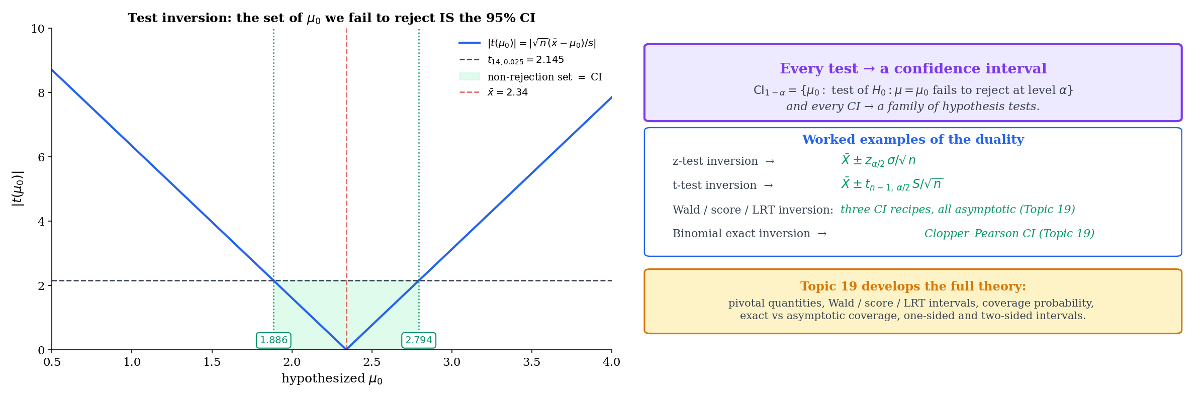
Fix a level . For each candidate parameter value , construct the level- test of . The non-rejection set — the collection of values for which the observed data does not lead to rejection — is a confidence interval for :
The coverage for every , because the test controls Type I error at level uniformly over in each hypothesis direction. Conversely, any confidence interval gives a family of level- tests: reject iff .
The duality is more than a formal correspondence — it is a concrete construction. Inverting a z-test gives the z-interval; inverting a t-test gives the t-interval; inverting an LRT gives the profile-likelihood interval; inverting a score test gives the score interval. Topic 19 develops all four constructions.
Z-interval. For iid Normal data with known , the level- two-sided z-test fails to reject iff , i.e., iff
The non-rejection set is — the textbook z-confidence interval.
T-interval. For iid Normal data with unknown , the analogous inversion of the t-test gives
using the -quantile of the distribution. For and , — slightly larger than the of the z-interval, reflecting the extra variability introduced by estimating .
The inversion also works for the Wald, score, and LRT tests in §17.9, giving three different intervals for a general parameter. Topic 19 develops the full set; for now, the preview is that the same machinery we just built handles both “is ?” and “what values of are plausible?”.
The t-interval works because the quantity is a pivot — its distribution () does not depend on any unknown parameter. The confidence interval is formed by inverting a distributional statement about the pivot. Pivots are available for the location-scale families (Normal, exponential with known rate, etc.) and give exact small-sample confidence intervals.
When pivots are not available (most general parametric models), we invert asymptotic tests instead: the Wald interval uses ; the score interval uses the set ; the LRT interval uses the set . All three have coverage asymptotically; their finite-sample coverage can differ substantially — the Wald interval is notoriously under-covering in small samples near the boundary (e.g., for binomial with near 0 or 1; the Wilson interval, based on the score test, is preferred). Full theory, with coverage diagnostics and comparisons, is Confidence Intervals & Duality (Topic 19).
17.11 Where the Framework Falls Short
Classical hypothesis testing is a tightly specified decision procedure, and it fails to answer several questions that practitioners often want it to answer. An honest account lists the failure modes.
A p-value tests whether the data are consistent with a specific null model. It does not rank competing models, and it does not quantify which model predicts better out of sample. An analyst who runs two separate hypothesis tests (one on each model) and picks the one with smaller p-value has not performed model comparison — they have performed two inconsistent Type I error controls and then post-selected. For genuine model comparison, use cross-validation, AIC, BIC, or held-out likelihood. Cross-validation is the ML-native standard; AIC and BIC are the frequentist and Bayesian large-sample approximations to out-of-sample predictive performance. The contrast is developed in Topic 24’s CV/IC framework and at formalml’s formalML: Model comparison .
The Bayesian analog of a hypothesis test is the Bayes factor
the ratio of marginal likelihoods under the two hypotheses. A Bayes factor of 10 is commonly interpreted as “strong evidence for ”; combined with a prior odds , it gives the posterior odds. Bayes factors are more consistent with Fisher’s “evidence” framing and less vulnerable to the Ioannidis critique (Remark 6), but they require specifying priors for the competing hypotheses, which introduces its own modelling choices. Bayesian Foundations (Topic 25) introduces the marginal likelihood and names Bayes factors; the full Bayes-factor framework and BMA are Topic 27’s territory.
Running independent tests, each at level , under independence produces an overall false-positive rate — which exceeds rapidly: at and , the overall rate is . Modern A/B testing platforms run thousands of simultaneous tests; naive per-test level control would give mostly false positives. Bonferroni correction (test each at level to control family-wise error at ) is the classical fix; Benjamini-Hochberg’s false discovery rate (FDR) controls the proportion of rejections that are false positives, with less power loss than Bonferroni at large . The full treatment is Multiple Testing & False Discovery (Topic 20), which addresses the “garden of forking paths” concern flagged in Remark 6.
Some replication-crisis concerns are not technical at all. A researcher who tests multiple hypotheses but reports only the significant one has inflated the effective Type I rate, and no multiple-testing correction can recover the right level if the correction isn’t applied. The remedy is pre-registration: announcing the hypotheses, the analysis plan, and the stopping rule before seeing the data. Adversarial collaboration extends this by recruiting a skeptic as a co-author, tasked with anticipating and pre-committing to the interpretation of each possible outcome. Both are non-technical but important complements to the multiple-testing machinery of Topic 20.
17.12 Summary & Forward Look
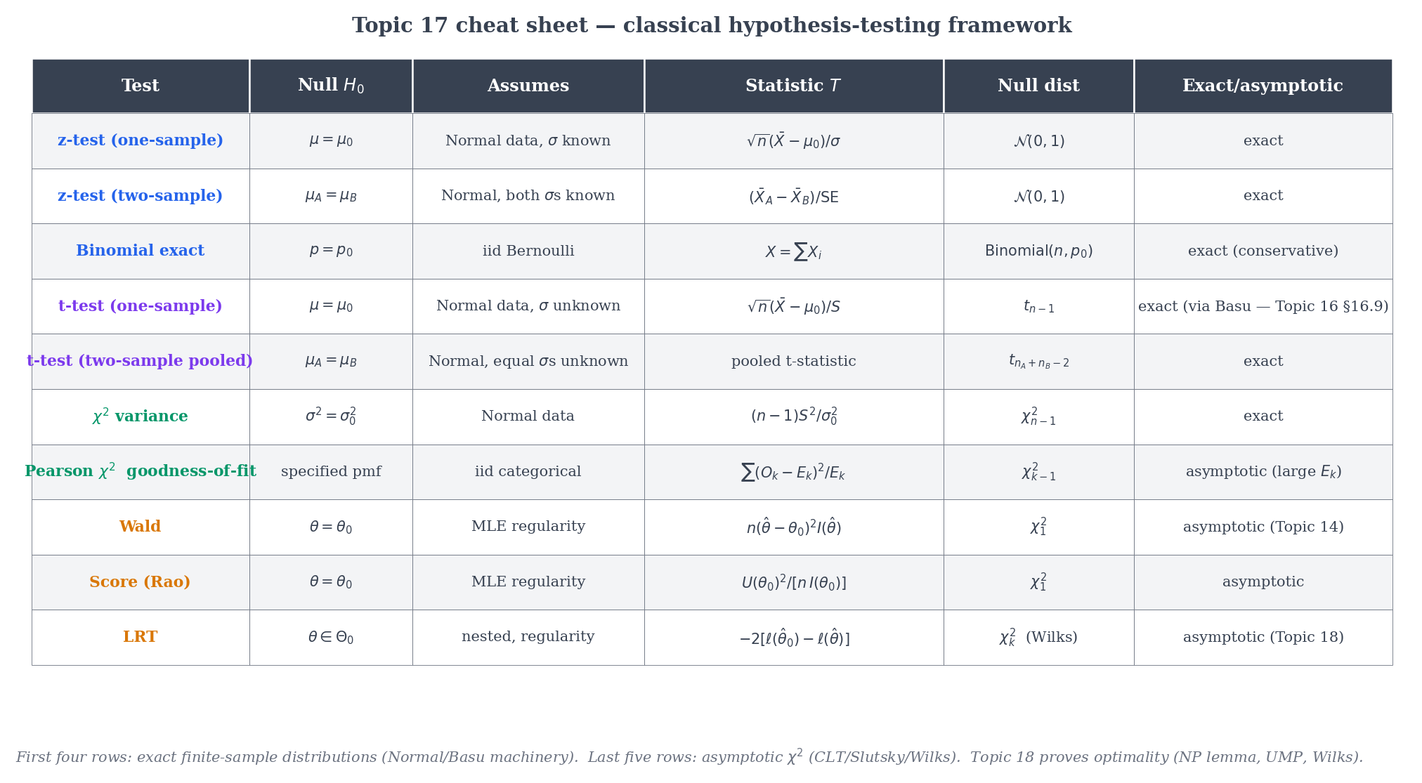
A compact map of the test families we have met.
| Test | Null | Assumes | Statistic | Null distribution | Exact or asymptotic? |
|---|---|---|---|---|---|
| z-test (one-sample) | Normal, known | Exact (Normal); asymptotic (general) via CLT | |||
| z-test (two-sample) | Both Normal, known | Exact under Normal; asymptotic via CLT | |||
| Two-proportion z | Large , | Asymptotic | |||
| Binomial exact | Bernoulli | Exact (discrete) | |||
| t-test (one-sample) | Normal, unknown | Exact via Basu | |||
| t-test (two-sample pooled) | Both Normal, unknown | Pooled t | Exact under equal variance | ||
| Welch t | Both Normal, unequal variances | Welch t | (Satterthwaite) | Asymptotic | |
| variance | Normal | Exact | |||
| Pearson (GoF) | Fixed cell probs | Multinomial, | Asymptotic | ||
| Wald | Regular MLE | Asymptotic | |||
| Score (Rao) | Regular MLE | Asymptotic | |||
| LRT | Wilks’ regularity | Asymptotic |
The two “exact” entries (z-test with known; t-test and variance under Normality) owe their exactness to the special structure of the Normal family — in particular, to Basu’s theorem (Topic 16 §16.9) giving .
Topic 17 set up the framework. The next three topics complete Track 5:
- Likelihood-Ratio Tests & Neyman-Pearson (Topic 18) — the optimality theory. Neyman-Pearson’s lemma: the LRT is UMP for simple-vs-simple. Uniformly most powerful tests, monotone likelihood ratio families, Wilks’ theorem proved in full, the three asymptotic tests’ finite-sample power compared.
- Confidence Intervals & Duality (Topic 19) — the duality previewed in §17.10 becomes the construction. Pivotal quantities, Wald / score / LRT intervals, coverage diagnostics, the Wilson interval for binomial proportions (which fixes the Wald boundary problem from Remark 13).
- Multiple Testing & False Discovery (Topic 20) — family-wise error (Bonferroni, Holm, Šidák, Hochberg), false discovery rate (Benjamini-Hochberg with full proof, Benjamini-Yekutieli for arbitrary dependence, Storey adaptive q-values), simultaneous CIs dualizing the FWER procedures, and the replication-crisis framing in quantitative terms. Track 5 closes here.
Beyond Track 5, the framework reappears in Linear Regression (F-tests §21.8 Thm 9, partial F-tests Example 8, ANOVA Example 9), Generalized Linear Models (Wald / score / LRT tests for GLM coefficients; the score test is the standard specification test), Bayesian Foundations (Topic 25) (posterior over , conjugate priors, credible intervals, Bernstein–von Mises; Bayes factors named in §25.10 with full development deferred to Topic 27), and Nonparametric Inference (permutation tests, rank tests, Kolmogorov-Smirnov). Finally, forward to formalML: A/B testing platforms , where every deployed experimentation system is running variants of Topic 17’s machinery at scale — and increasingly augmenting them with sequential-testing, variance-reduction (CUPED), and always-valid-inference extensions.
The shift from estimation to testing — from “best guess” to “decide” — is the conceptual move. Every topic in Track 5 and beyond builds on the scaffolding we put up here.
References
- Erich L. Lehmann & Joseph P. Romano. (2005). Testing Statistical Hypotheses (3rd ed.). Springer.
- George Casella & Roger L. Berger. (2002). Statistical Inference (2nd ed.). Duxbury.
- Ronald A. Fisher. (1922). On the Mathematical Foundations of Theoretical Statistics. Philosophical Transactions of the Royal Society A, 222, 309–368.
- Jerzy Neyman & Egon S. Pearson. (1933). On the Problem of the Most Efficient Tests of Statistical Hypotheses. Philosophical Transactions of the Royal Society A, 231, 289–337.
- ‘Student’ (William Sealy Gosset). (1908). The Probable Error of a Mean. Biometrika, 6(1), 1–25.
- Karl Pearson. (1900). On the Criterion that a Given System of Deviations from the Probable is Such that It Can Be Reasonably Supposed to Have Arisen from Random Sampling. Philosophical Magazine (5th series), 50, 157–175.
- Abraham Wald. (1943). Tests of Statistical Hypotheses Concerning Several Parameters When the Number of Observations is Large. Transactions of the American Mathematical Society, 54(3), 426–482.
- C. Radhakrishna Rao. (1948). Large Sample Tests of Statistical Hypotheses Concerning Several Parameters with Applications to Problems of Estimation. Mathematical Proceedings of the Cambridge Philosophical Society, 44(1), 50–57.
- Samuel S. Wilks. (1938). The Large-Sample Distribution of the Likelihood Ratio for Testing Composite Hypotheses. Annals of Mathematical Statistics, 9(1), 60–62.
- Ronald L. Wasserstein & Nicole A. Lazar. (2016). The ASA’s Statement on p-Values: Context, Process, and Purpose. The American Statistician, 70(2), 129–133.
- John P. A. Ioannidis. (2005). Why Most Published Research Findings Are False. PLoS Medicine, 2(8), e124.
- Andrew Gelman & Eric Loken. (2013). The Garden of Forking Paths: Why Multiple Comparisons Can Be a Problem, Even When There is No ‘Fishing Expedition’ or ‘p-Hacking’. Department of Statistics, Columbia University.