Method of Moments & M-Estimation
Moment matching, the sandwich variance, and robust estimation — the framework that unifies MoM, MLE, and modern robust statistics.
15.1 From Matching Moments to Estimating Equations
Topic 14 gave us a recipe — write down the likelihood, find its peak — that produces an estimator with the best possible asymptotic variance under regularity. Before that recipe existed, statisticians had a different one. Karl Pearson, working in the 1890s on biometric data and trying to fit mixtures of two Normal distributions to crab measurements, observed that the parameters of a model are functions of its moments. So estimate the moments from the data, plug those estimates into the inverse function, and you have an estimator. The procedure is called the method of moments, abbreviated MoM, and it is the oldest estimation principle in modern statistics.
The mechanics are disarmingly simple. If are an iid sample from a distribution with parameter , and the population moments are known functions of for , then the sample moments are estimators of by the law of large numbers. Setting them equal and solving the resulting system
gives the MoM estimator . There are no derivatives, no iterations, no convexity arguments — just the inverse of the moment map.
The first systematic use of moment matching appears in Pearson’s 1894 paper “Contributions to the Mathematical Theory of Evolution,” where he fit a mixture of two Normals to the carapace-width measurements of 1000 crabs from the Bay of Naples. The mixture has five parameters — two means, two variances, and a mixing weight — so Pearson computed five sample moments and solved the resulting nonlinear system, by hand, to recover the underlying components. He used the method because no other recipe existed. The likelihood-maximization principle was still nearly thirty years away.
The reason MoM predates the MLE is operational. Until R. A. Fisher’s 1922 paper “On the Mathematical Foundations of Theoretical Statistics,” likelihood was viewed as one of several plausible criteria for fitting a distribution; there was no general argument for preferring it. What Fisher established — that the MLE is consistent, asymptotically Normal, and asymptotically efficient under regularity — required machinery (Fisher information, the Cramér–Rao bound, asymptotic theory) that did not exist in Pearson’s era. So a calculation that could be done won out over one that would have required theory not yet developed. The lesson is durable: even today, when the MLE is intractable, MoM is the first thing to reach for.
The catch — and it is a real one — is that MoM is almost never as good as the MLE in the asymptotic sense. The next eleven sections develop both the recipe and the diagnostic comparison. We will see that for the natural exponential families (§7), MoM coincides exactly with the MLE; outside that boundary, MoM trades efficiency for simplicity, and the trade is sometimes severe (Gamma shape, where MoM extracts only ~68% of the available information at ) and sometimes catastrophic (Cauchy, where MoM has nothing to match because the population mean does not exist). The framework that unifies all of this — both MoM and MLE — is M-estimation, the topic of §15.9–§15.11.
15.2 The Method-of-Moments Principle
The construction is straightforward but worth stating with care, because the moment map can be invertible globally, locally, or not at all, and the difference matters.
For an iid sample , the -th sample moment is
The first sample moment is the sample mean (Definition 13.2). By the strong law of large numbers, whenever the population moment exists.
Let be iid from a parametric family with , and write for the -th population moment as a function of . Suppose the moment map
is invertible on its image. The method-of-moments estimator is the (unique) solution to the system of equations
Equivalently, .
The moment map is the bridge between parameter space and observable space, and the MoM estimator is what we get when we cross the bridge in the opposite direction from how the model is usually specified. Forward: moments. Backward: sample moments .
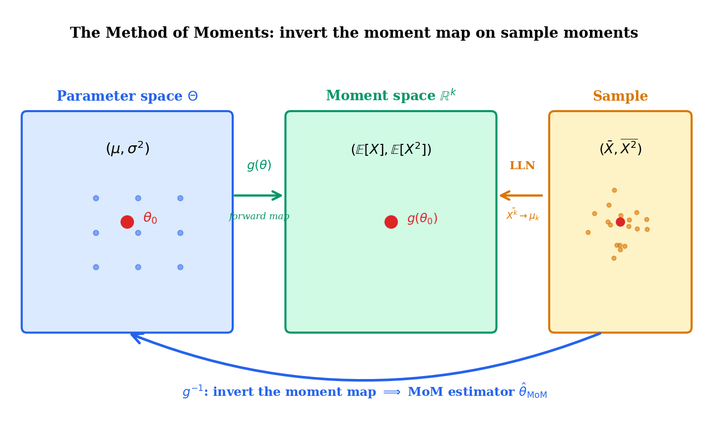
If the moment map is continuous and one-to-one on , and lies in the image , then the MoM estimator exists and is unique. If is continuously differentiable with a non-singular Jacobian at the true parameter , then the inverse is differentiable in a neighborhood of , and is well-defined for sufficiently large with probability tending to one.
The two regularity conditions — invertibility of and non-singularity of its Jacobian — are exactly what we need for the asymptotic theory in §15.5 to go through. When they fail (mixtures with non-identifiable components; the Cauchy distribution, where is not even defined), MoM fails. We catalogue those failure modes in §15.6.
For , the first two population moments are
Setting and and solving:
and
The MoM variance estimator is the biased form (the same form the MLE uses, see Example 14.2), not the Bessel-corrected form. This is structural: MoM matches the population variance to the raw second-moment-minus-squared-first-moment, whose unbiased correction is a shift. We will see in §15.7 that for the Normal variance, — they are the same estimator, both dominated in MSE by the unbiased .
For , . So , giving
This is identical to the MLE (Example 14.7). The reason — to be made precise in Theorem 5 of §15.7 — is that the Exponential is an exponential family in its natural parameter, and for such families the MLE is a moment-matching estimator. The two recipes coincide.
For , . So
again identical to the MLE. The Poisson is also a natural exponential family. The pattern will become explicit in §15.7.
The construction in Definition 2 uses exactly moment equations to identify parameters. If we attempted to use more — say, the first three sample moments to estimate two parameters — the system is over-determined and generally has no exact solution. Choosing which two equations to enforce, or how to weight all three, is the move that takes us from MoM to the generalized method of moments (GMM, Hansen 1982). We preview GMM in §15.12. For the rest of this topic, we hold to the exact-identification setting: moments for parameters.
15.3 Scalar Examples: Uniform, Bernoulli, Geometric
Three scalar-parameter examples deepen the intuition. The Uniform case is the cautionary one: MoM is much worse than the MLE.
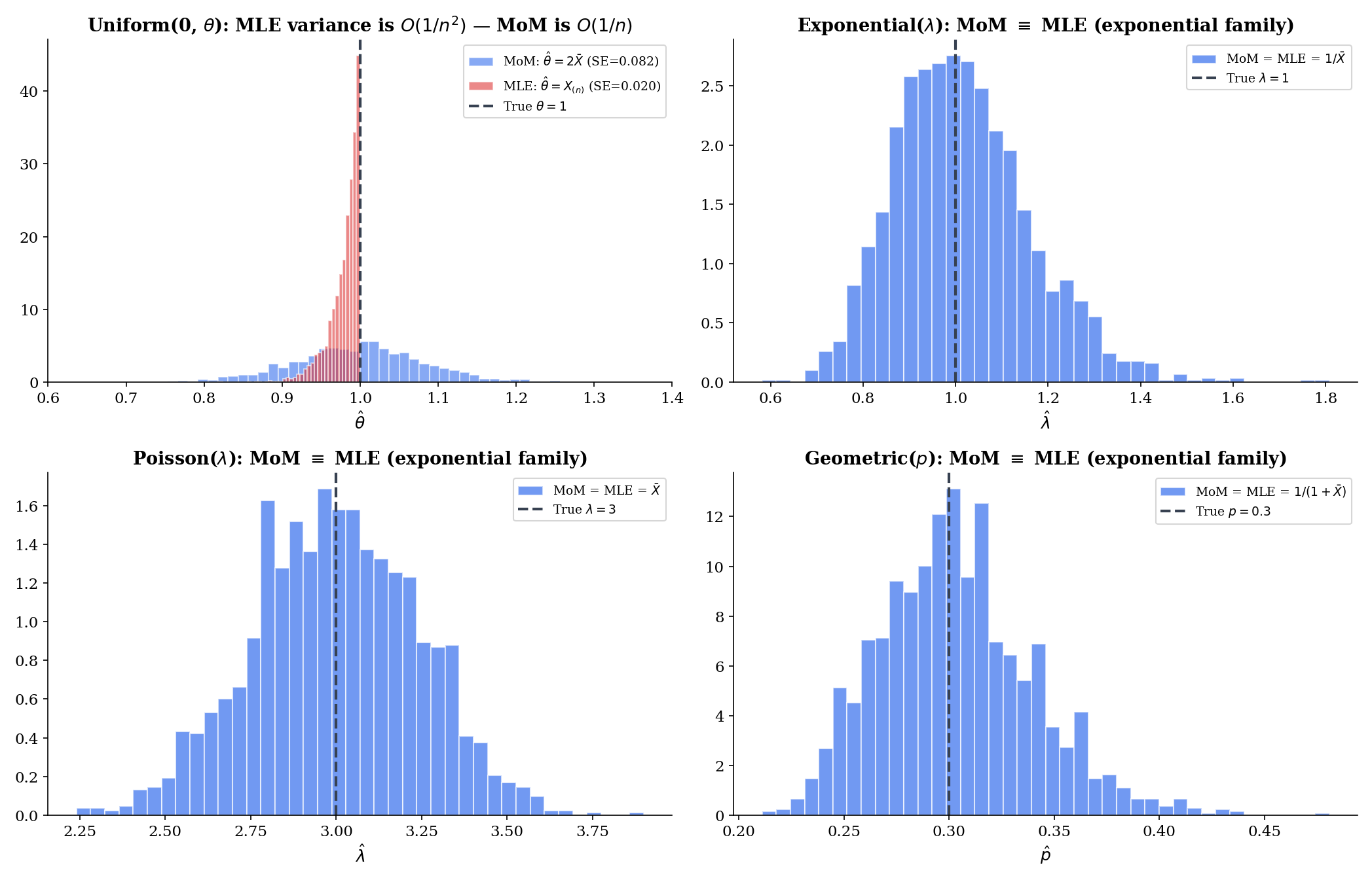
For , . So , giving
This is a perfectly reasonable estimator — consistent, with asymptotic variance from the delta method. But it has two pathologies that the MLE does not. First, with positive probability , where is the largest observation. That is impossible — the parameter must be at least as large as every observed value, so is infeasible. Second, the MLE for this problem is
with asymptotic variance of order — a full order of magnitude better than MoM’s . The ratio as .
We do not call this a failure of MoM — MoM gives an answer, and the answer converges to . We call it the most graphic illustration of why efficiency matters: when the MLE achieves a faster convergence rate (here vs. ), the asymptotic ratio of variances is not a fixed number but a sequence going to zero.
For , , so
The Bernoulli is yet another natural exponential family, so MoM = MLE. Three for three so far in the exponential-family column.
The Geometric distribution comes in two conventions; we adopt the failures-before-first-success convention with and . Then , and setting gives
If instead we use the trials-until-first-success convention with , then and . Both are exponential families; both coincide with the MLE.
Example 4 hinted at it; the issue is general. The MoM estimate is the inverse moment map applied to sample moments, which can land anywhere in — not just in . A few realistic ways this bites:
- Negative variance. For a Gamma sample, requires . With probability one this holds for and a non-degenerate sample, but a near-constant sample (small ) makes the estimate explode.
- Probability outside [0, 1]. For a Beta, the MoM solves where ; if the formal MoM gives , outside the parameter space.
- Mixing weight outside [0, 1]. Pearson’s two-Normal mixture famously yielded mixing weights below 0 and above 1 on certain datasets — Pearson reported this as a feature of the data (“the model is mis-specified”) rather than a bug of MoM.
The standard fix is to project onto the constraint set, but at that point we have abandoned pure MoM. Better diagnostic: when MoM gives an absurd answer, suspect the model.
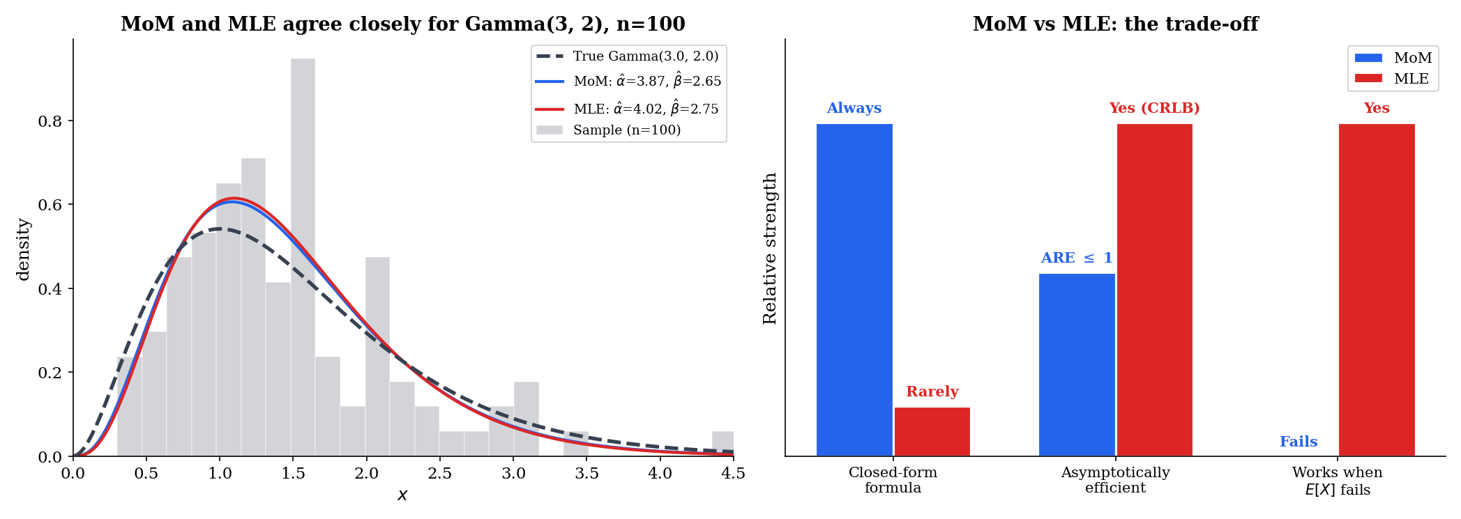
1.49450.869215.4 Multivariate MoM: The Two-Parameter Gamma
The Gamma distribution with shape and rate is the canonical example of a continuous family where MoM has a clean closed form and the MLE requires Newton-Raphson. Both estimators recover consistently, but the MoM gets there in two lines of algebra. This contrast — algebraic simplicity for MoM, iterative computation for MLE — is the heart of why MoM remains useful.
For a model with parameters , the moment map is the vector of population moments,
Its Jacobian at is the matrix
The MoM estimator is , well-defined when is invertible at the true parameter.
For the Gamma, the moments are well-known:
It is more convenient to work with the variance alongside the mean. Setting and (with the biased sample variance from §15.2) and dividing the first by the second,
and then
Closed form, two lines. The MLE for the Gamma shape, in contrast, has no closed form: the score equation involves the digamma function , which has no algebraic inverse. Topic 14 §14.7 walked through the Newton-Raphson solution.
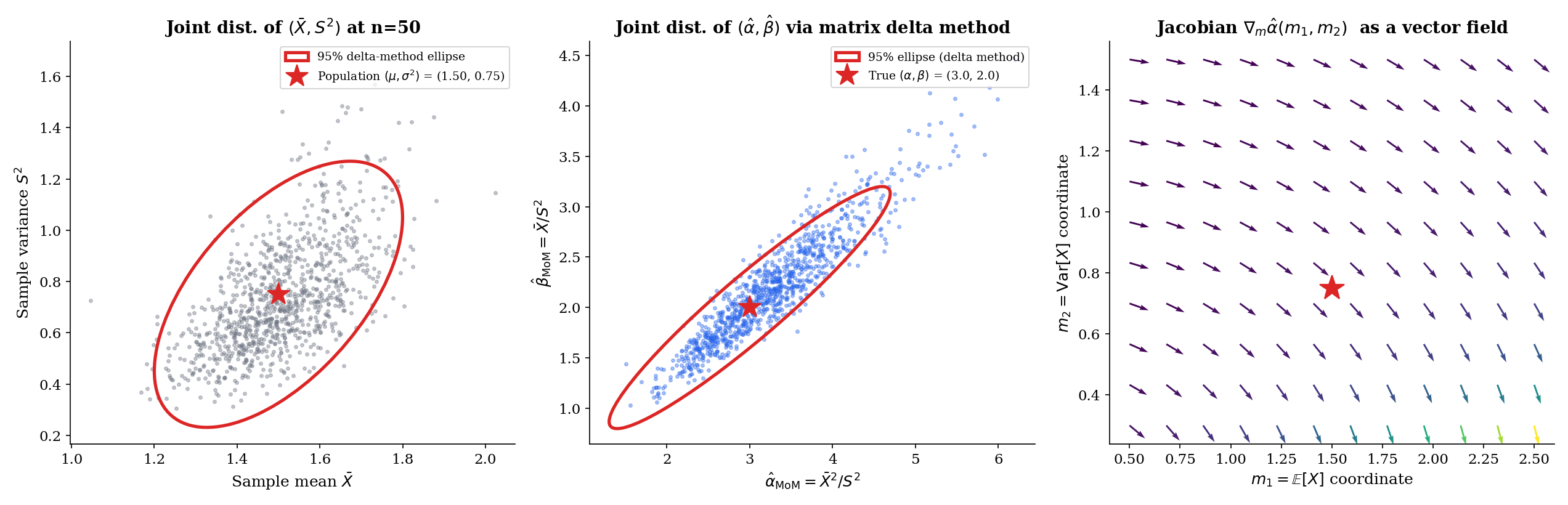
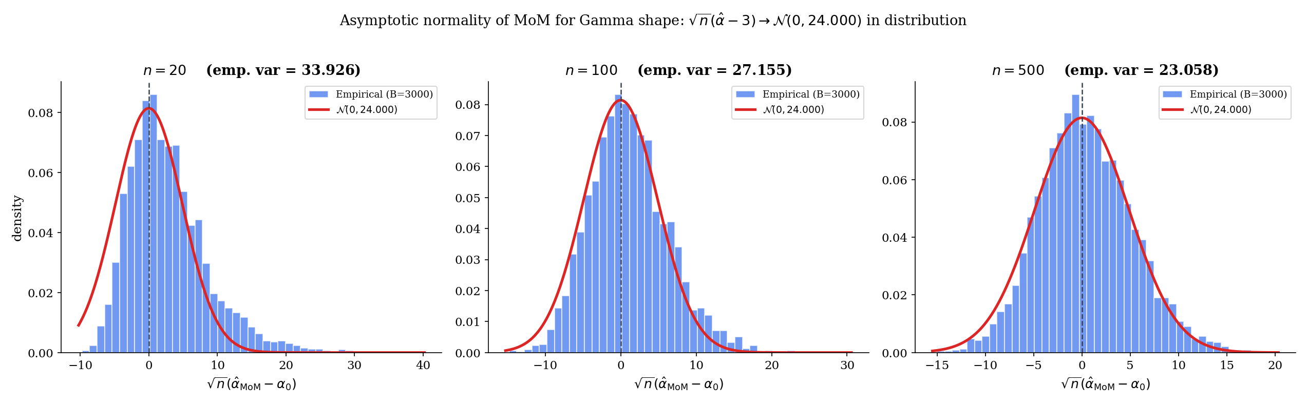
Let be iid with , and let , . Then
and
where is the limiting covariance of given by the multivariate CLT, and is the Jacobian of the moment map.
Proof [show]
We apply the matrix delta method (Theorem 11.9, multivariate form) to the moment-to-parameter map.
Step 1 — joint asymptotic Normality of the sample moments. The pair for each is iid with mean and covariance matrix where
By the multivariate CLT (Topic 11 §11.8) applied to the iid pairs,
Step 2 — invertibility of the moment map. The map has Jacobian
Its determinant evaluates to for , so is locally invertible at every interior point. The inverse is continuously differentiable in a neighborhood of .
Step 3 — apply the delta method. Writing for the inverse map and for its Jacobian (by the inverse function theorem),
Since and , this is the asymptotic-normality claim with covariance .
Step 4 — consistency from the SLLN. The sample moments converge a.s. to the population moments by the strong LLN (Topic 10 §10.5). Continuity of at together with the continuous-mapping theorem (Topic 11 §11.4) gives
This establishes both consistency and asymptotic normality. ∎ — using the multivariate CLT (§11.8), the delta method (§11.9), and the continuous-mapping theorem.
Restating from the derivation above: for iid ,
where is the biased (1/) sample variance — the same form used by the MLE for the Normal variance, and the form that makes the MoM and the maximum-likelihood approach align as cleanly as possible. With samples from , the typical estimate sits within ±0.1 of on a single replicate. The MLE for is more accurate by a factor of in standard error (the ARE = 0.68 of §15.7); whether that matters depends on the application.
For , the mean and variance are
A short manipulation yields
with the same biased sample variance. The MLE for the Beta has no closed form — the score equations involve digamma functions — so the gap in computational cost is genuine. We will see in §15.8 that fitting a Beta in scipy or R uses the MoM estimate as the warm start for the MLE iteration.
15.5 Consistency and Asymptotic Normality of MoM
Theorem 2 made the multivariate Gamma case rigorous. The general multivariate-MoM theorem is the same proof with the model-specific moments and Jacobian replaced by abstract symbols.
Let be iid from a model with parameter . Suppose:
- The first population moments exist and are continuous in .
- The moment map is one-to-one on , and is continuous on a neighborhood of .
Then as .
The proof is one line: by the SLLN (componentwise), and converges a.s. to by continuity of and the continuous-mapping theorem (Topic 11 §11.4).
The asymptotic-normality theorem requires more.
Under the conditions of Theorem 3, additionally suppose:
- (finite higher moments — needed for the CLT to apply to sample moments).
- The moment map is continuously differentiable in a neighborhood of with non-singular Jacobian .
Then
where is the covariance matrix of under .
Proof [show]
The proof generalizes Steps 1–3 of Proof 1 (Theorem 2) with the Gamma-specific computations replaced by abstract symbols.
Step 1 — joint asymptotic Normality of sample moments. The vector is iid across with mean and covariance matrix whose entry is . Finite ensures has finite entries. The multivariate CLT (Topic 11 §11.8) then gives
Step 2 — apply the delta method. Let . By the inverse function theorem (formalcalculus: differentiation), is continuously differentiable in a neighborhood of with Jacobian . The multivariate delta method (Topic 11 §11.9) then transforms the asymptotic distribution of the sample moments through :
Since applied to the sample moments is , and applied to the population moments is , this is the claimed limit. ∎ — using the multivariate CLT (§11.8), the delta method (§11.9), and the continuous-mapping theorem.
The four assumptions of Theorem 4 are exactly the ingredients the proof needs. (1)–(2) are the identification assumptions: the moments exist and the moment map distinguishes parameters. (3) is the Lyapunov-style higher-moment assumption that lets the CLT apply componentwise to the iid moments . (4) is the smoothness assumption that lets the delta method propagate the limit through . When any of these fails — most notably (1) for Cauchy and (3) for heavy-tailed Pareto — MoM does not just have a worse asymptotic variance; it has no asymptotic variance, because the underlying CLT does not apply. We see those failure modes in §15.6.
The Exponential MoM is . By Theorem 4 with and the delta method on ,
Computing: , so ; and . Hence
The Cramér–Rao lower bound for the Exponential rate (Example 13.10) is — exactly what we just computed. So the Exponential MoM is asymptotically efficient, achieving the CRLB. This is the §15.7 statement that the MoM matches the MLE for natural exponential families, made concrete.
15.6 When the Method of Moments Fails
The conditions of Theorem 4 can fail in three structurally different ways. Each illuminates the moment-matching principle from the negative side.
A distribution has finite -th moment if . When , the -th moment does not exist (in either the abstract or the practical sense), the SLLN does not apply to , and the MoM equation has no meaningful right-hand side. The MoM estimator is then undefined, not merely badly behaved.
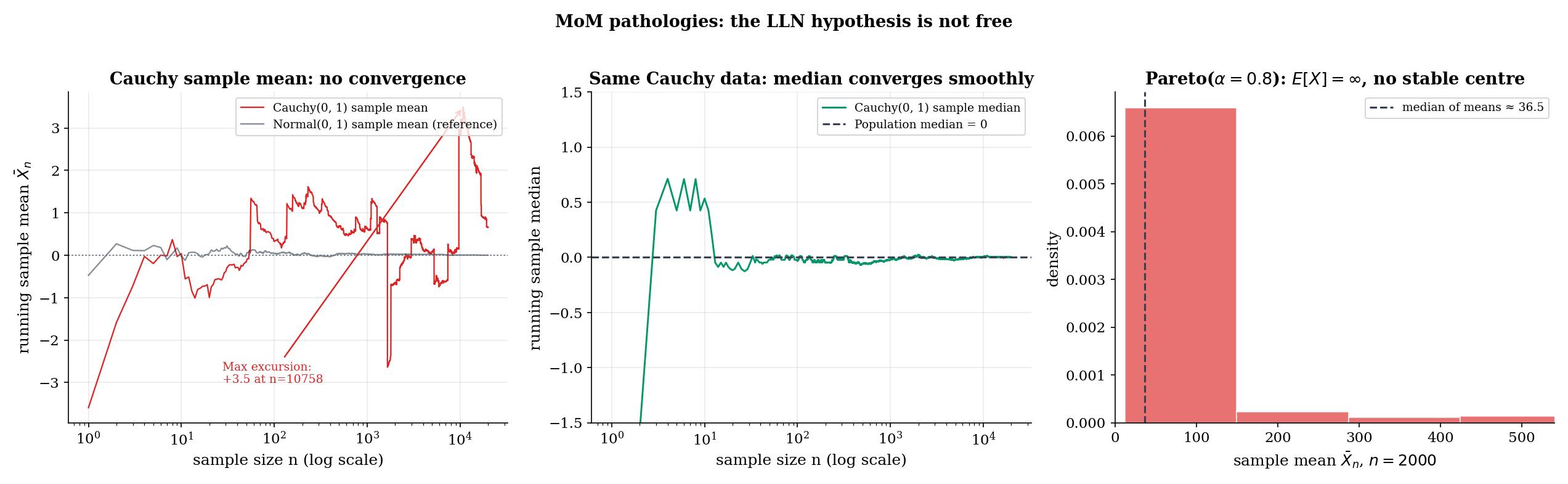
The Cauchy distribution with location and scale 1 has density . Its tails are , so
i.e., and the population mean does not exist. The MoM equation has a left-hand side that does not converge as : the sample mean of Cauchy data exhibits wild excursions at every scale — large jumps appear with positive probability at every , so the sequence has no limit (almost surely it does not converge).
The MLE, by contrast, is consistent. The log-likelihood
is twice continuously differentiable, has a unique maximum (the MLE solves a polynomial equation in of degree when expanded), and the Fisher information is finite. The MLE is asymptotically Normal with variance . Cauchy is the cleanest example of MoM failing while MLE succeeds: the population mean does not exist, but the population is fully identified by the location of its peak — and the likelihood sees the peak.
The Pareto distribution with shape and scale has density for . Its first moment is
which converges only when , in which case . For , , and the MoM moment-matching equation has no consistent population side. Empirically, for Pareto data does not converge but instead grows roughly like — heavy-tailed extremes pull it up at every sample size.
The MLE for the Pareto is closed-form: , and is consistent with finite asymptotic variance, regardless of whether . So once again — even more cleanly than Cauchy — the MoM fails because does not exist, while the MLE works because the log-transformed data has finite moments.
Consider the mixture model — equal mixing weights, common mean zero, two variance components. The first three population moments are
Only the second moment depends on . The first moment is identically zero (by symmetry), and the third moment is identically zero (by symmetry of each Normal component). So the moment map is invertible only if we use the second moment — and it has dimension 1 in moment space, embedded in 3-dimensional moment space. With three moments and one parameter, MoM is over-determined; with one moment and one parameter, MoM works trivially.
The deeper issue surfaces when we try to estimate more parameters in the mixture — say, both variances and the mixing weight. With two distinct components having equal means, the moment system collapses: the same set of population moments is consistent with a continuum of parameter combinations. The moment map is not invertible. MoM fails because the model is not identifiable from moments alone. The MLE faces the same issue — but the MLE has access to the full likelihood, which uses the shape of each observation’s contribution and can identify the components even when their moments coincide.
The pattern in Examples 10–12 is general. When MoM fails, it fails visibly: an undefined limit, an estimate outside the parameter space, or a system that simply has no unique solution. This is, perversely, a strength — MoM tells you when it has failed, often more loudly than the MLE does. If or on real data, the appropriate response is not to project the estimate onto the constraint set but to ask whether the model is right.
0.000. Maximum absolute excursion of the running mean (so far): 1.69.The MoM equation X̄n = μ1(θ̂) has nothing to match — there is no population moment to converge to.
15.7 Asymptotic Relative Efficiency: MoM vs MLE
The reason MoM coincides with the MLE for the Exponential (Example 2) and Poisson (Example 3) is structural — those families admit a representation in which the MLE is a moment-matching estimator. The reason MoM diverges from the MLE for the Gamma shape is also structural — the Gamma is an exponential family, but only the rate is in the natural parameter; the shape requires a different sufficient statistic. We make this rigorous now.
For two consistent, asymptotically Normal estimators and of the same parameter , with asymptotic variances and , the asymptotic relative efficiency of relative to is
When this ratio is less than 1, is asymptotically less efficient than . ARE = 1 means the two estimators are asymptotically equivalent. (Definition 13.13 of Topic 13.)
Let be a -parameter exponential family in natural parameter form,
with sufficient statistic and log-partition function . The MLE satisfies
This is exactly the moment-matching equation: is the population mean of the sufficient statistic, so the MLE equates the model’s expected sufficient statistic to the sample average — which is the MoM equation when the sufficient statistics are the moments. In particular, for distributions whose sufficient statistic is (Exponential, Bernoulli, Poisson), the MLE is the moment-matching estimator , so .
The proof is the one-line argument from Topic 7 §7.8: differentiating with respect to and setting the result to zero gives . By the well-known identity (a moment-generating-function calculation, also Topic 7 §7.8), this is moment matching.
For iid , with the MoM estimator and the MLE from the score equation, the asymptotic variances are
and (from the inverse Fisher-information matrix at )
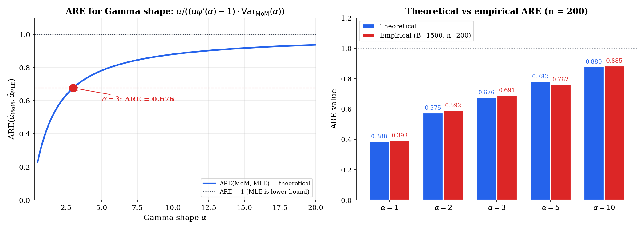
where is the trigamma function. Therefore
The MoM asymptotic variance comes from Theorem 4 with the Gamma-specific and from the proof of Theorem 2. The MLE asymptotic variance comes from inverting the Fisher information matrix at and reading off the entry. The ratio is what we plot.
At : the trigamma function evaluates to , so . Then
The Monte Carlo verification at over 1000 replications gives an empirical — consistent with the theoretical 0.676 to within Monte-Carlo noise. So the MLE extracts about 1/0.68 ≈ 1.47 times as much information from each observation as MoM does — equivalently, MoM needs 47% more data to match MLE precision.
The Exponential family has , so by Theorem 5, the MLE coincides with the MoM. Asymptotic variance for both is (per Example 9), and exactly. This is not approximate equality — the two estimators are the same function of the data. They cannot have different asymptotic variances.
Three reasons, in increasing order of importance.
(1) Closed form. When the moment map inverts in elementary functions — Gamma, Beta, Weibull (numerically), Pareto with — MoM gives an estimate in two lines of arithmetic. No iteration, no convergence diagnostics, no risk of missing a local maximum.
(2) Warm-start for MLE. The next section makes this precise. When MLE requires Newton-Raphson, the MoM estimate is almost always a good starting point: it is consistent (so it converges to at the same rate as the MLE), it is computable, and it lies inside the parameter space whenever the data are not pathological. Newton from MoM converges in 3–5 iterations at typical ; Newton from an arbitrary start can take 8–12 or fail to converge at all.
(3) Diagnostic. When MoM and MLE disagree wildly, the model is suspect. The two recipes use different summaries of the data — sample moments for MoM, the full likelihood for MLE — and a large discrepancy means the model is not capturing the moment structure consistently with the likelihood structure. This is a free goodness-of-fit signal, available without additional computation.
15.8 MoM as a Warm-Start for MLE
Topic 14 §14.7 introduced Newton-Raphson for the Gamma shape MLE. It mentioned, briefly, that “a standard initial guess is the method-of-moments estimate” — that’s the warm-start pattern. Here we make it first-class.
The MLE is asymptotically efficient. The MoM is consistent. The two estimates converge to the same true at the same rate, and the difference between them is . So the MoM estimate places us, with high probability, within an neighborhood of the MLE — close enough that one or two Newton steps land at the MLE to machine precision. This is the algorithmic reason MoM matters even when we have decided to fit by maximum likelihood.
The conceptual analogue in optimization is multi-resolution: solve a cheap approximate problem to get a good initial point, then refine with the expensive exact procedure. MoM-warm-started MLE is exactly this pattern at the level of statistical estimation.
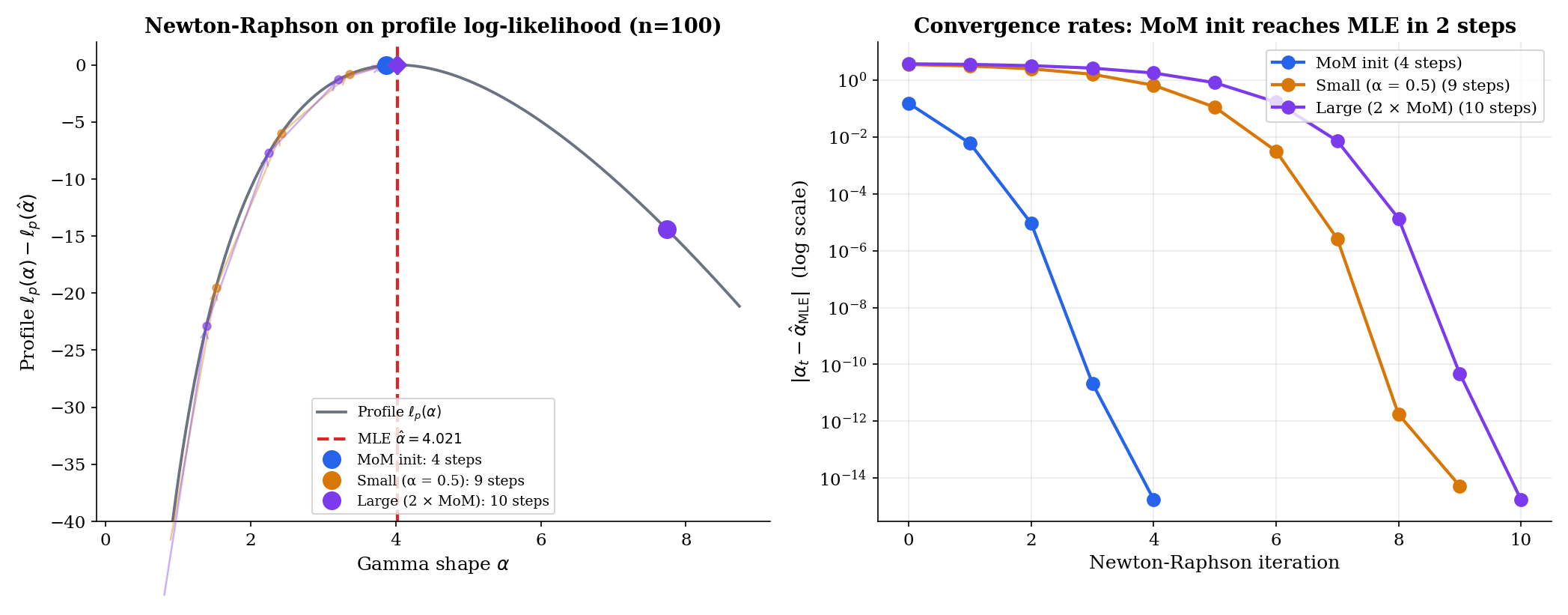
For a sample of size , the MoM estimate of the shape is typically on a single replicate. Starting Newton-Raphson on the score equation from this initial value, convergence to machine precision (step size ) requires 4 iterations in the typical case. Starting from takes 9 iterations — Newton has to traverse the steep left tail of the score function. Starting from takes 10 iterations, with the first step often overshooting. The pattern holds across sample sizes from to : MoM-warm-started Newton converges in 3–5 steps; arbitrary-start Newton needs 8–12.
This is not a textbook idea waiting to be implemented. It is the dominant pattern in the actual codebases that fit distributions to data.
- scipy.stats.fit: when a parametric family is specified, scipy first computes a MoM estimate (it calls this “method of moments” internally), then refines via L-BFGS or a Nelder–Mead simplex on the negative log-likelihood. MoM is the explicit default initial point.
- R’s MASS::fitdistr: the same pattern. MoM init, then
optim()for the MLE. - Statsmodels (Python): iteratively reweighted least squares for GLMs, with the OLS estimate (a MoM-like start) as the initial guess.
The dominant alternative — searching for a starting point by random restart or by grid search — is much slower and rarely necessary when MoM is available. The exceptions are models where MoM is undefined (mixtures with non-identifiable components, latent-variable models) or pathological (Cauchy). For everything else, MoM is the warm-start.
3.4198 · α̂_MLE = 3.3870 · Steps: MoM init 4, small init 7, large init 7.15.9 M-Estimation: The Unifying Framework
Both MoM and MLE produce an estimator by setting an empirical sum to zero. For MLE, the sum is the score: , where . For MoM, the sum is a moment residual: . The shared structure is
for some choice of estimating function . The framework that takes this structure as primary is called M-estimation, and it gives a single asymptotic theory for all such estimators — including MoM, MLE, OLS, the Huber location estimator, the median, and quantile regression.
Let be iid from a distribution with parameter . Given an estimating function satisfying the moment condition at the true parameter, the M-estimator is any solution of the estimating equation
Existence and uniqueness require regularity on (e.g., monotonicity in , or strict convexity of an associated loss); see van der Vaart Chapter 5 for the formal conditions.
When for some scalar loss function , the M-estimator is equivalently the minimizer of the empirical risk:
In this gradient form, the estimating equation is the first-order condition for the minimization. The label Z-estimator (for “zero” of the estimating equation) is sometimes reserved for the general form even when no underlying loss exists; M-estimator (for “minimum” of an empirical risk) emphasizes the loss-function origin.
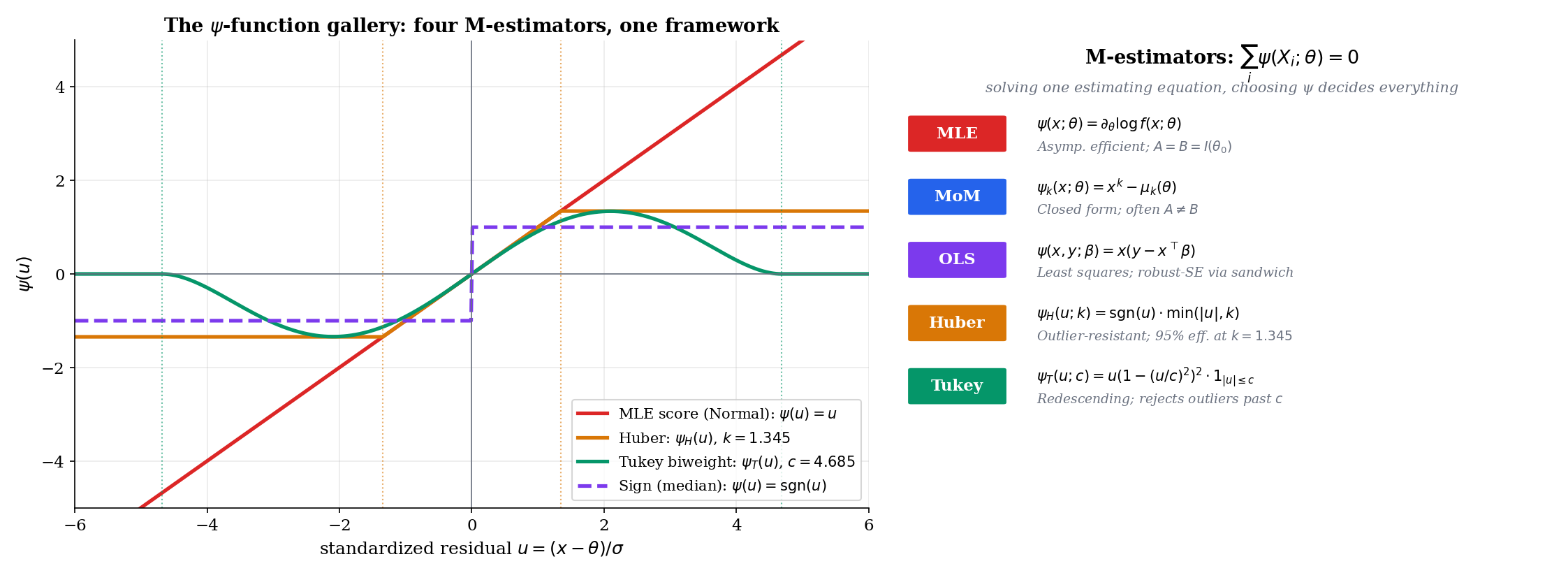
For an iid sample from a parametric family , the maximum-likelihood estimator is the M-estimator with estimating function
The moment condition holds because the population score has mean zero (Theorem 13.8). The associated loss is the negative log-density: , with the minimizer of the negative log-likelihood.
For a -parameter model with first population moments , the method-of-moments estimator is the M-estimator with vector-valued estimating function
The moment condition holds at the true parameter by definition. There is no associated loss function in general — MoM is a Z-estimator, not an M-estimator in the strict loss-minimization sense.
For a regression model with , the ordinary least-squares estimator is the M-estimator with
The moment condition holds by the regression assumption. The loss is . We develop OLS in detail in Linear Regression; here it suffices to note that OLS, MLE for a Normal-error linear model, falls into the M-estimation framework.
The list extends. Quantile regression: . Generalized linear models: is the score of the GLM likelihood. Robust regression: is a Huber or Tukey choice. The unifying observation is that the estimator is determined by the choice of , and the asymptotic theory is the same in every case — the sandwich variance of §15.10.
15.10 Asymptotic Theory of M-Estimators: The Sandwich Variance
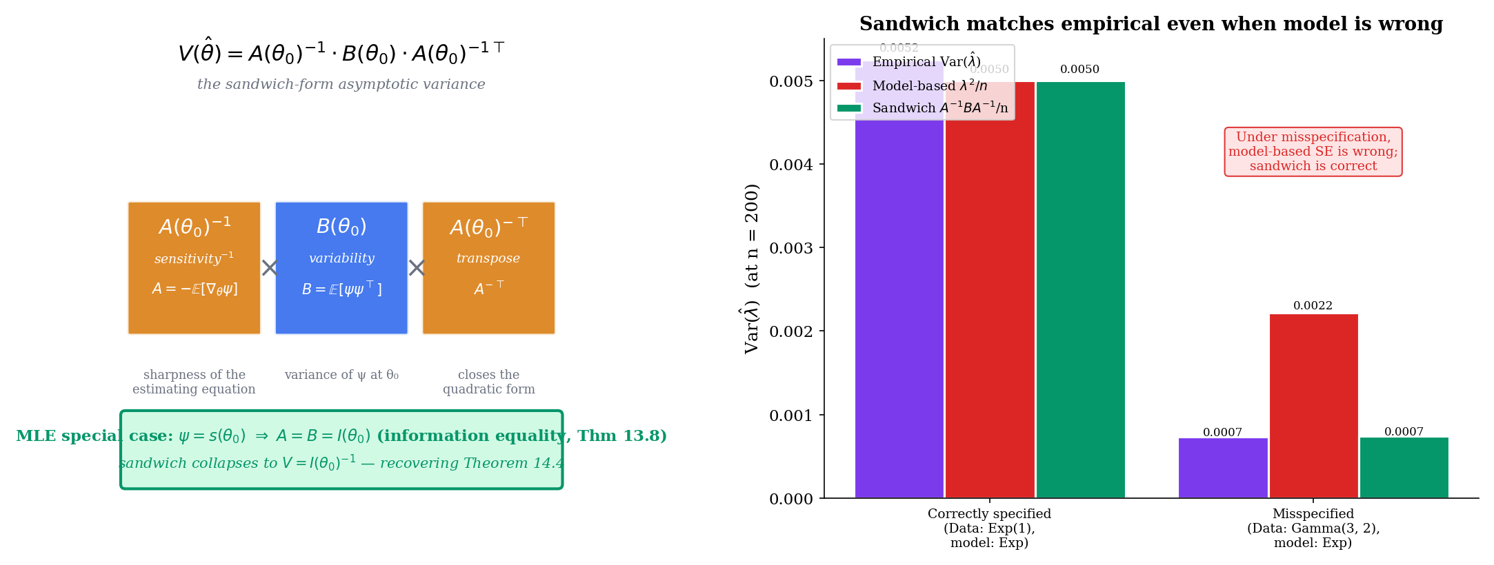
The single theorem in this section is, structurally, the most consequential in the topic. It generalizes the asymptotic-normality result for the MLE (Theorem 14.4) to every M-estimator, and it produces an asymptotic variance — the sandwich form — that reduces to the Fisher-information inverse in the MLE case but differs from it whenever the model is misspecified.
For an M-estimator with smooth estimating function , define
the sensitivity matrix — how strongly the population estimating function responds to changes in . And define
the variability matrix — the covariance of at (using the moment condition to drop the mean). When is scalar, both and are scalars; for vector , they are matrices.
Sign conventions vary across references. We adopt the convention that is positive definite in the regular case (so the negative sign appears explicitly). The alternative convention flips the sign and treats as negative definite.
Under suitable identifiability and regularity conditions on (e.g., is uniquely zero at and continuous in a neighborhood, plus uniform convergence of to its expectation), the M-estimator satisfies
The argument parallels the MLE consistency proof (Theorem 14.3): uniform LLN on , plus the unique-zero hypothesis, plus a continuity argument.
Under the conditions of Theorem 9 plus continuous differentiability of in near , finite second moments of , and invertibility of ,
where the asymptotic variance is the sandwich form
For scalar this reduces to .
When is the score function of a correctly specified parametric model, (information equality, Theorem 13.8), the sandwich collapses to , recovering the MLE asymptotic variance of Theorem 14.4 as a corollary.
Proof [show]
This is the core asymptotic theorem of M-estimation. The argument is a Taylor expansion of the estimating equation around , followed by a one-step rearrangement and an application of the LLN, the CLT, and Slutsky’s theorem.
Step 1 — Taylor expand the estimating equation. By assumption (Theorem 9), so for large , lies in a neighborhood of where is differentiable. Taylor-expanding around :
for some on the line segment between and (a multivariate mean-value form).
Step 2 — solve for the deviation. Assuming is invertible for large (which it is, with probability tending to one, by the invertibility assumption on and the consistency ),
Multiplying both sides by :
We will compute the limit of each factor separately.
Step 3 — the denominator. By the LLN applied to the iid , plus uniform convergence in a neighborhood and the consistency ,
Step 4 — the numerator. The iid random vectors have mean zero (the moment condition) and finite covariance (by the second-moment assumption). By the multivariate CLT (Topic 11 §11.8),
Step 5 — combine via Slutsky. Slutsky’s theorem (Topic 11 §11.4) lets us multiply the convergent-in-probability denominator by the convergent-in-distribution numerator:
A linear transformation of a Normal vector is Normal with covariance :
Step 6 — MLE collapse. When is the score of a correctly specified model, the information equality (Theorem 13.8) states
so , and the sandwich variance collapses:
This is exactly the MLE asymptotic variance from Theorem 14.4. The MLE asymptotic-normality theorem is the special case of the M-estimator asymptotic-normality theorem. ∎ — using the multivariate CLT (§11.8), the LLN (Topic 10), Slutsky (§11.4), and the information equality (Theorem 13.8).
For any correctly specified parametric family with score , the M-estimator with has by the information equality. The sandwich variance is . Theorem 14.4 is recovered as a corollary of Theorem 10. The Fisher-information inverse is the correct-model asymptotic variance; the sandwich is the general one.
For Exponential data, MoM uses . Compute:
(With the sign convention from Definition 8 — note that here is the convention warning we flagged.) And
Sandwich: . This matches the asymptotic variance derived in Example 9 via the delta method. The two routes — applying Theorem 4 (delta method) and applying Theorem 10 (sandwich) — agree, as they must.
A demonstration of the misspecified case is more striking. Suppose we generate data from but fit it as an Exponential, treating as the estimating equation. The MoM estimate converges to , not to any “true” Exponential rate (there is none). The model-based asymptotic variance would be at . But the empirical variance over Monte Carlo replicates is — three times smaller than the model-based guess, because the Gamma distribution has lower variance than the Exponential at the same mean. The sandwich estimate, which uses the empirical and computed from the actual Gamma data, is , matching the empirical to three significant figures. This is the practical significance of : it is the signature of model misspecification, and the sandwich formula corrects for it.
The information equality is a theorem under correct specification — and only under correct specification. When the model is wrong, and generally differ, and the sandwich variance gives the asymptotic variance of the M-estimator under the true (mis-specified) data-generating distribution rather than under the postulated (mis-specified) model.
This has a name in econometrics: robust standard errors, or White’s heteroskedasticity-consistent standard errors for OLS — exactly the sandwich formula applied to OLS under heteroskedasticity. The model-based standard errors assume homoskedasticity (and hence ); the sandwich corrects for the violation. Linear Regression develops this fully. The M-estimation framework makes the correction transparent: it is not a separate “robust” trick; it is what happens when you take the asymptotic theory seriously.
15.11 Robust M-Estimation: Huber and Tukey
The estimating-function in M-estimation is a design — choose it to balance efficiency under the postulated model against robustness to deviations from that model. The MLE choice ( score) is the one extreme: maximally efficient when the model is correct, but fragile under contamination. Two alternatives, both due to mid-20th-century work in robust statistics, give controlled trade-offs.
Huber’s ψ-function with tuning constant is
The associated loss function is for , and for — quadratic in the central region, linear in the tails. The Huber location estimator solves for a robust scale (typically the MAD, ).
The default choice gives 95% asymptotic efficiency under Normal data while bounding the influence of any single observation.
Tukey’s biweight ψ-function (also called the bisquare) with tuning constant is
The associated loss is bounded:
Tukey’s is redescending — it rises in the central region, peaks, and returns to zero outside . Observations beyond standardized residuals get weight exactly zero and are entirely ignored. The default gives 95% asymptotic efficiency under Normal data, with full rejection of outliers beyond .
![Three panels. Left: ψ_H(u; k = 1.345) — linear with slope 1 in [−1.345, 1.345], then flat at ±1.345 in the tails. Center: ψ_T(u; c = 4.685) — bell-shaped on [−4.685, 4.685], rising from 0 at u = 0, peaking near |u| = c/√3, then descending to 0 at u = ±c, and identically zero beyond. Right: estimator variance versus contamination fraction for the sample mean (rises sharply), the median (flat), Huber (flat through ~10%, then rising), and Tukey (flat well past 10%).](/images/topics/method-of-moments/huber-vs-tukey.png)
Among all M-estimators of location with bounded influence function, the Huber estimator with tuning constant chosen to match a specified Normal-efficiency target is minimax: it minimizes the maximum asymptotic variance over the class of -contaminated Normal distributions
for a corresponding . The choice corresponds to roughly contamination tolerance and 95% efficiency under pure Normal.
The proof, due to Huber (1964), is a saddle-point argument: the worst case in is a heavy-tailed Normal-like distribution, and the optimal estimator under that worst case turns out to be the Huber location with tuning depending on . This was the founding result of robust statistics — it gave a principled recipe for outlier-resistant estimators, replacing earlier ad-hoc procedures like trimmed means and Winsorization.
Generate samples: 180 from and 20 from (that is, 10% contamination at ). The sample mean is — pulled away from the true location 5 by the outliers. The median is — unmoved. The Huber location with and MAD scale gives as well — also unmoved, but with smaller variance than the median when the contamination is not present (when contamination is zero, the Huber matches the mean almost exactly because no observations are clipped).
Tukey’s redescending goes one step further. Beyond , , so the corresponding observations make no contribution to the estimating equation — they are effectively discarded. On the same contaminated sample as Example 18, Tukey gives with the variance of the median, but with somewhat better efficiency at the clean center because the central kernel is smoother.
The cost of the redescending shape is a concavity issue: is not monotone in , so the iteratively-reweighted fixed-point iteration can converge to a local optimum. The standard fix is to start from the median (which is consistent and globally well-defined), then refine to the Tukey estimate.
The (asymptotic) breakdown point of an estimator is the largest fraction of the sample that can be replaced by arbitrary outliers without making the estimate go to infinity. Formally,
where is the set of distributions within -contamination of . The maximum possible breakdown point is — any larger allows the contaminated distribution to be the majority, in which case identifying the “true” parameter is impossible.
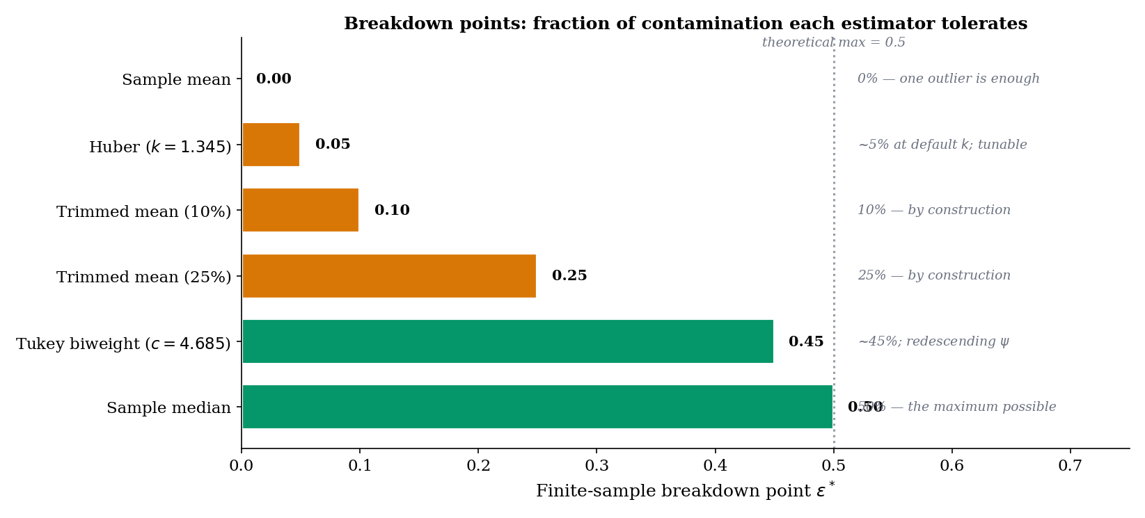
The figure above uses the older convention of reporting Huber and Tukey’s minimax-contamination tolerances rather than their asymptotic breakdown points. With a robust scale like the MAD, both Huber and Tukey achieve the maximum breakdown point of 1/2 (Rousseeuw–Leroy 1987) — the same as the median. The 5% bar for Huber should be read as: under the minimax-optimal tuning, the estimator is designed to be near-efficient against an contamination class. Empirical drift past ~10–20% in finite samples is a separate, gentler phenomenon driven by corruption of the MAD itself.
The breakdown points for common location estimators are:
- Sample mean. . A single outlier at sends the mean to .
- Sample median. . Up to nearly half the sample can be arbitrarily corrupted before the median becomes undefined; the median is the optimum in this sense.
- Huber location at , paired with a robust scale (MAD). . Asymptotically, the Huber-with-MAD estimator achieves the maximum breakdown point — the same as the median (Rousseeuw–Leroy 1987, §1). The often-quoted figure is a different quantity: the contamination level for which the default is minimax-optimal under Huber’s gross-error model. In practice the estimator drifts gradually as grows, well before the asymptotic 1/2 is reached, because at high contamination the MAD itself becomes corrupted.
- Tukey biweight at . (asymptotic). Redescending — once outliers are far enough out, they have zero weight, so increasing the fraction further does not move the estimate (until the redescending region itself becomes the majority of the data, at which point the estimator can have multiple local optima).
- -trimmed mean. . Trim the top and bottom observations and average the rest; the breakdown is exactly the trimming proportion.
The default is not arbitrary. It is the value that makes the asymptotic variance of the Huber location, under pure data, exactly times the asymptotic variance of the sample mean (which is 1 under unit-variance data) — that is, 95% efficiency under the Normal model. Bounded influence: the maximum value caps the impact of any single observation. The combination — 95% efficiency on a clean sample plus bounded influence on contaminated samples — is the dominant default in modern robust regression. Tukey’s is the analogous value for the biweight, giving the same 95% efficiency under Normal.
Why 95% and not, say, 99%? The reasoning is empirical: pushing efficiency above 95% (with small) makes the estimator behave nearly identically to the mean in the central region, surrendering most of the robustness. Pushing efficiency below 95% (with small) gains additional outlier resistance but at noticeable efficiency loss on clean data. The 95% point is roughly the elbow of this trade-off curve.
15.12 Summary & Forward Look: GMM and Beyond
The method of moments matches sample moments to population moments and solves; the M-estimation framework generalizes by replacing the moment-matching equation with a more general estimating equation . The asymptotic theory is uniform across the framework: consistency from a uniform LLN, asymptotic normality from a Taylor expansion plus the CLT, and asymptotic variance in the sandwich form that collapses to the Fisher-information inverse when is the score under correct specification. Choosing differently — Huber, Tukey, the score, the moment residual — produces a universe of estimators with controllable trade-offs between efficiency under the postulated model and robustness against deviations from it.
| Property | Method of Moments | Maximum Likelihood | General M-Estimator |
|---|---|---|---|
| Estimating equation | |||
| Closed form | Often (Gamma, Beta, Pareto with ) | Rare (only for exponential families with closed-form inverse ) | Depends on |
| Consistency | Yes if invertible, exist | Yes under standard regularity | Yes under Theorem 9 conditions |
| Asymptotic variance | (sandwich) | ||
| Asymptotic efficiency | MLE for natural exponential families; MLE in general | Yes (achieves CRLB) | Yes only under correct specification with score |
| Robustness to outliers | Poor (sample moments are non-robust) | Poor (likelihood is non-robust) | Tunable via (Huber, Tukey) |
| Computational cost | Closed-form: . Iterative: | Newton-Raphson: , typically iter = 4–10 | Depends on |
The method of moments uses exactly moment equations to identify parameters. Generalized method of moments (GMM), introduced by Lars Peter Hansen in his 1982 Econometrica paper, lifts this restriction: it allows moment conditions on parameters, giving an over-identified system that is then solved by minimizing a weighted distance.
Specifically, given moment conditions with the population property , define the empirical moment vector
The GMM estimator with weighting matrix (an positive-definite matrix that may depend on the data) is
When and , GMM reduces to ordinary MoM. When , the estimator is over-identified: the moment conditions cannot all be satisfied exactly, so GMM finds the that comes closest in the -weighted norm. The optimal weighting matrix — the one that minimizes the asymptotic variance of — is , the inverse of the covariance matrix of the moment conditions. This is efficient GMM.
GMM is the workhorse of empirical economics: it covers instrumental variables (IV) estimation, Euler equation estimation in dynamic consumption models, asset-pricing moment conditions, and the Arellano-Bond estimator for dynamic panels. The asymptotic theory parallels M-estimation but with the additional weighting-matrix layer. We do not develop GMM further in formalStatistics; the natural home is a future econometrics topic. For the canonical reference, see Hansen (1982).
Where this leads. Sufficient Statistics extends Topic 13’s evaluation framework with the Rao-Blackwell theorem and Lehmann–Scheffé, comparing UMVUE to both MLE and MoM; when MLE and MoM coincide (exponential families), they are both UMVUE under completeness. Hypothesis Testing builds the score test and Wald test as asymptotic tests (Topic 17 §17.9); the sandwich-variance estimator developed in §15.10 reappears as the basis of robust hypothesis tests under model misspecification in Track 6 (Linear Regression; Generalized Linear Models). Confidence Intervals inverts the M-estimator asymptotic-normality result: a Wald-type interval is , with the sandwich-variance estimate. Linear Regression treats OLS as the M-estimator with ; White’s heteroskedasticity-consistent standard errors are exactly the sandwich formula applied to OLS. Generalized Linear Models develops the Huber and Tukey extensions of OLS — robust regression — built on §15.10–§15.11.
Across formalML, M-estimation organizes much of supervised learning. formalML: Empirical Risk Minimization is M-estimation — the empirical risk is the average loss, and minimizing it solves a Z-estimating equation. formalML: Robust Statistics develops the Huber and Tukey M-estimators in regression, with the influence-function machinery and breakdown-point analysis built atop §15.11. formalML: Quantile Regression adopts the check-loss ψ-function, a non-smooth instance of the framework. And formalML: Generalized Method of Moments extends MoM to the over-identified setting Hansen (1982) introduced.
The reader who has worked through Topics 13–15 has the complete classical estimation toolkit: an evaluation framework (Topic 13), a maximally efficient default estimator (Topic 14), a fast warm-start with closed-form structure for many families (Topic 15 first half), and a unifying asymptotic theory that subsumes everything and accommodates robust alternatives (Topic 15 second half). Track 4 closes with Sufficient Statistics (Topic 16), which gives the data-reduction theory completing the foundations.
References
- Casella, G., & Berger, R. L. (2002). Statistical Inference (2nd ed.). Duxbury.
- van der Vaart, A. W. (1998). Asymptotic Statistics. Cambridge University Press.
- Hampel, F. R., Ronchetti, E. M., Rousseeuw, P. J., & Stahel, W. A. (1986). Robust Statistics: The Approach Based on Influence Functions. Wiley.
- Rousseeuw, P. J., & Leroy, A. M. (1987). Robust Regression and Outlier Detection. Wiley.
- Lehmann, E. L., & Casella, G. (1998). Theory of Point Estimation (2nd ed.). Springer.
- Wasserman, L. (2004). All of Statistics. Springer.
- Hansen, L. P. (1982). Large Sample Properties of Generalized Method of Moments Estimators. Econometrica, 50(4), 1029–1054.
- Huber, P. J. (1964). Robust Estimation of a Location Parameter. Annals of Mathematical Statistics, 35(1), 73–101.