Bayesian Computation & MCMC
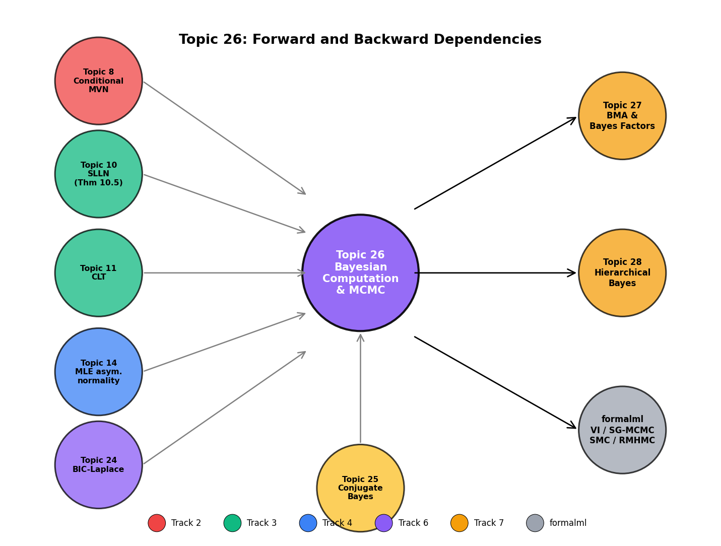
Topic 25 handed us the Bayesian framework but stopped at the conjugate families. Every non-exponential-family likelihood, every hierarchical prior, every mixture model has a posterior known only up to the intractable normalizing constant m(y). Topic 26 develops the Monte Carlo machinery that makes Bayesian inference operational in those regimes: Metropolis–Hastings proved correct via detailed balance (featured), Gibbs sampling as a special case, Hamiltonian Monte Carlo with leapfrog, NUTS (Hoffman–Gelman 2014), the R̂ and ESS convergence diagnostics, and the Markov-chain ergodic theorem that generalizes Topic 10's iid SLLN (Thm 10.5) to dependent sequences.
26.1 When conjugacy fails
Topic 25 built the Bayesian framework on a load-bearing simplification: the prior and likelihood live in matching conjugate families, so the posterior has a closed form. Five canonical pairs cover much of applied statistics — Beta-Binomial, Normal-Normal, Normal-Normal-Inverse-Gamma, Gamma-Poisson, Dirichlet-Multinomial — and every conjugate analysis looks the same: observe data, update hyperparameters, read off credible intervals from the named family.
But the conjugate framework fails whenever the likelihood is not exponential-family (logistic regression with a Gaussian prior, robust regression with a Student-t likelihood), whenever the prior is hierarchical (school effects inside a group-level Normal, shrinkage priors like the horseshoe), or whenever the model has many parameters (mixture models, hidden Markov models, anything with latent variables). The posterior is still well-defined — Bayes’ theorem is one line — but the normalizing constant
is a high-dimensional integral without a closed form. We know only up to this unknown constant.
The trick underneath every MCMC algorithm: we never need . To sample from we only need ratios (in the MCMC-theory notation introduced in §26.3, where denotes the posterior-as-target), and the unknown cancels from numerator and denominator. This is the structural reason every MH / HMC / NUTS algorithm moves by proposing a candidate and comparing its unnormalized density to the current state’s.
Topic 26 develops four algorithms end-to-end: Metropolis–Hastings (§26.2, the featured recipe), Gibbs sampling (§26.3, the conjugate-full-conditional specialization), Hamiltonian Monte Carlo (§26.4, the gradient-aware extension), and the No-U-Turn Sampler (§26.5, the self-tuning HMC default that Stan and PyMC ship). Convergence diagnostics follow in §26.6. The theoretical spine is §26.7’s Markov-chain ergodic theorem, which generalizes Topic 10’s Theorem 10.5 (Kolmogorov/Etemadi SLLN) from iid sequences to dependent Markov chains. Ten specializations and alternatives — adaptive MCMC, reversible-jump, Riemann-manifold HMC, stochastic-gradient MCMC, sequential Monte Carlo, variational inference, parallel tempering, nested sampling, Bayesian nonparametric MCMC, slice sampling — each get a forward-pointing paragraph in §26.10, not a dedicated section. Topic 26’s bar is pedagogical: does this method change how the reader thinks about proposals, acceptance, or convergence?
MCMC is asymptotically exact: under irreducibility, aperiodicity, and positive recurrence, long-run chain averages converge almost surely to posterior expectations (§26.7 Thm 5). The price is computational — chains take time to mix, and diagnosing convergence is an empirical art. Variational inference trades exactness for speed (§26.10 Rem 26); Topic 26 commits to the exactness side of the trade.
26.2 Metropolis–Hastings
The Metropolis–Hastings (MH) algorithm is the pedagogical kernel of the entire topic. Every subsequent algorithm is a specific choice of proposal kernel inside the MH frame — Gibbs is MH with acceptance , HMC is MH on an extended position–momentum state, NUTS is MH with an adaptive trajectory length. Getting the MH correctness proof right once buys the rest.
Let be a target density on , known up to a normalizing constant. A proposal kernel is a conditional density that generates a candidate given the current state . Given a proposal, the MH acceptance probability is
The MH transition kernel is
where the first term covers accepted moves and the second (the rejection mass ) parks the chain at when the proposal is rejected.
A distribution is invariant for a transition kernel if for every measurable . A sufficient condition for invariance is detailed balance: for all , where is the off-diagonal density of .
The MH transition kernel of Def 1 satisfies detailed balance with respect to . Consequently is invariant for .
Proof 1 Proof of Thm 1 (MH correctness, FEATURED) [show]
Step 1 — setup. Target density on , known up to a normalizing constant. Proposal density with the accessibility condition: whenever and is reachable. Acceptance probability
Transition kernel
Claim: is invariant for : for every measurable , .
Step 2 — strategy. Prove detailed balance for the off-diagonal density . Detailed balance implies invariance (MEY2009 Thm 1.6).
Step 3 — reduce to two cases. Let . By symmetry (swap ) one case suffices. Suppose . Then and .
Step 4 — LHS of detailed balance.
Step 5 — RHS of detailed balance.
LHS equals RHS. The case is the same calculation with labels swapped.
Step 6 — invariance from detailed balance. For any measurable ,
Apply detailed balance to the inner integral: . Substitute:
∎ — using the MH acceptance ratio definition (HAS1970 §2) and the detailed-balance-⇒-invariance lemma (MEY2009 Thm 1.6).
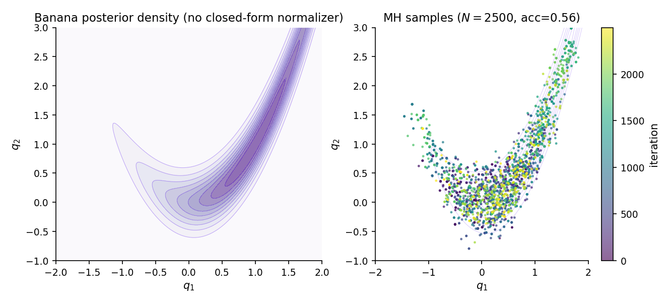
The canonical 2-D tuning problem. Target (Rosenbrock banana). Use a symmetric Gaussian proposal , so the proposal density ratio in drops out: . Start from , tune until the empirical acceptance rate approaches the optimum. The banana’s curved ridge is the difficulty — too-small leaves the chain sticky at the current point; too-large overshoots the ridge and rejects almost every proposal.
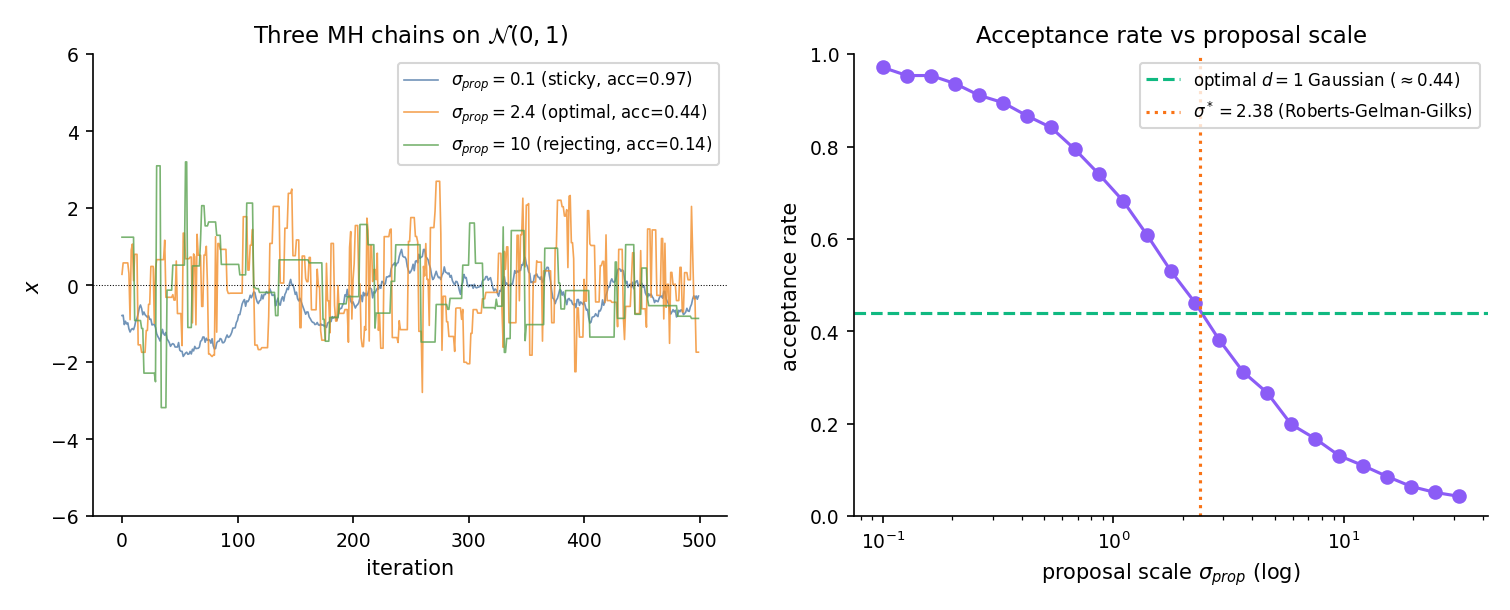
For a -dimensional Gaussian target with a Gaussian random-walk proposal of scale , Roberts–Gelman–Gilks 1997 proved the asymptotically optimal proposal covariance is , where is the target covariance. The induced optimal acceptance rate is 0.234 for and 0.44 for . ROB2004 Ch. 7 gives the full derivation. For Bayesian applications, the natural choice is , using Topic 14 Theorem 4 — MLE asymptotic normality tells us the posterior is approximately Gaussian at large , and its covariance is the inverse Fisher information scaled by .
When — a symmetric proposal, like a Gaussian random walk — the ratio and . This is the 1953 Metropolis recipe; Hastings 1970 generalized to asymmetric proposals.
The independence sampler uses a proposal that doesn’t depend on the current state — typically a Laplace approximation to the posterior. Acceptance ratio becomes , with the importance-ratio-like structure familiar from importance sampling. Works well when is a good global approximation; catastrophic when it misses modes.
Target acceptance 20–40% for random-walk Metropolis on smooth unimodal posteriors; larger is over-proposing, smaller is over-rejecting. Tune the proposal covariance to where available; otherwise use the empirical covariance of a pilot chain. The tuner component below lets you feel the acceptance-rate-vs-scale trade-off directly.
Geometric ergodicity — the rate of convergence to is exponential — requires compatible proposal and target tails (ROB2004 §7.3). Polynomial-tailed targets (Student- with few degrees of freedom, scale-mixture distributions) violate geometric ergodicity under Gaussian proposals; §26.8 Rem 21 names the standard mitigation (heavier-tailed proposals or reparameterization).
Canonical 1-D target. Roberts-Gelman-Gilks optimal scale 2.38 gives ~44% acceptance.
26.3 Gibbs sampling
Gibbs sampling is the special case of MH where the proposal is a draw from a full conditional distribution — the acceptance probability turns out to be identically 1, so every proposal is accepted. The algorithm is the practical pathway from Topic 25 §25.5’s five canonical conjugate pairs to posterior inference in hierarchical and mixture models: when a full joint posterior has a non-conjugate structure but every coordinate’s full conditional is conjugate, Gibbs lets us sample coordinate-by-coordinate using the closed-form updates we already know.
Track 7 notation was locked in Topic 25 §25.3; we inherit every symbol verbatim. Topic 26 adds seven symbols specific to Markov-chain Monte Carlo:
| Object | Symbol | Interpretation |
|---|---|---|
| Proposal density | MH proposal kernel: density of given current state . | |
| Acceptance probability | MH acceptance of given proposal from . | |
| Transition kernel | One-step chain kernel: accept-move density plus rejection mass on . | |
| Invariant distribution | Satisfies . In Bayesian use is the posterior; reconciles with Topic 25’s prior by context. | |
| Gelman–Rubin statistic | Multi-chain convergence diagnostic; as chains mix. | |
| Effective sample size | (ESS) | — iid-equivalent sample count for the chain. |
| Autocorrelation at lag | for fixed test function ; decays under geometric ergodicity. |
HMC uses for the position–momentum pair following Neal 2011 convention. The letter thus does double duty — proposal kernel in MH notation, position coordinate in HMC notation — but the distinction is unambiguous by context (function-of-two-arguments vs pair-of-vectors).
Let with joint target . The full conditional of coordinate is
where . The systematic-scan Gibbs sampler iterates: at iteration , for in sequence, draw .
The systematic-scan Gibbs sampler preserves . Equivalently: each coordinate-wise sub-step is an MH step with acceptance probability identically 1.
Proof 2 Proof of Thm 2 (Gibbs-as-MH) [show]
Step 1 — setup. State . Target with full conditionals .
Step 2 — the -th component update as MH. Propose with density
a proposal that only moves coordinate , drawing it from the target’s full conditional given the other coordinates held fixed.
Step 3 — factor the target. By the defining property of conditional densities,
Step 4 — acceptance ratio. Since on the non- coordinates,
So : every Gibbs proposal is accepted.
Step 5 — conclude. By Thm 1 (MH correctness), each full-conditional sub-kernel preserves . The systematic-scan Gibbs iteration is the composition , and composition of -preserving kernels is -preserving.
∎ — using Thm 1 (MH correctness) and the composition closure of -preserving kernels (MEY2009 §1.4).
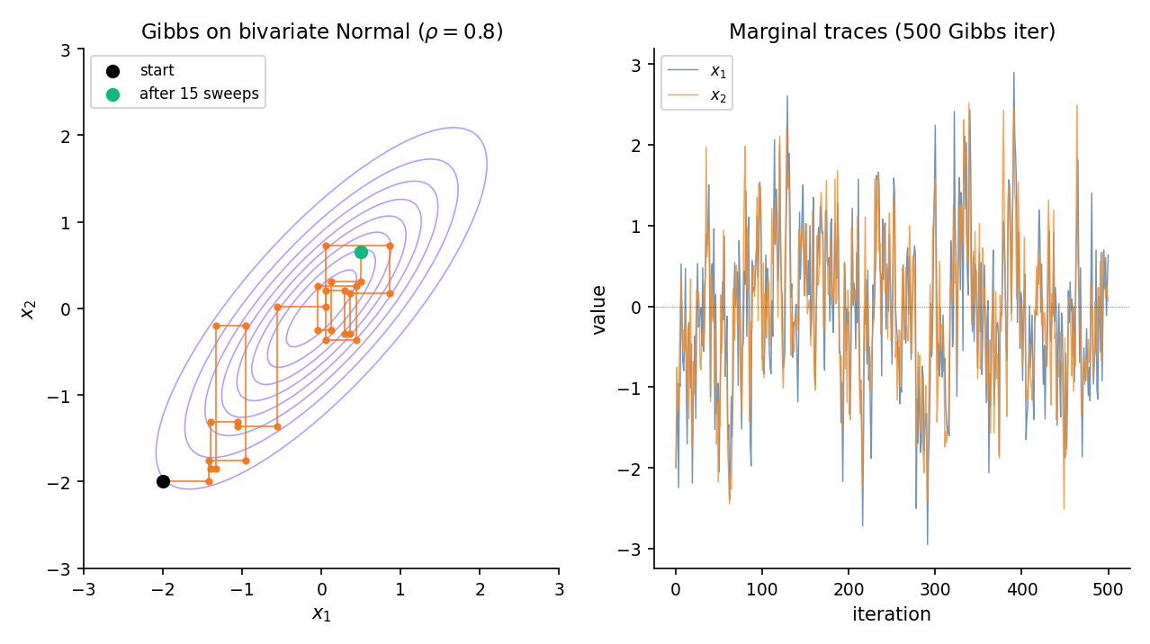
Let with \Sigma = \begin{psmallmatrix}1 & \rho \\ \rho & 1\end{psmallmatrix}. Topic 8 Theorem 3 — the conditional-MVN formula — gives the full conditionals in closed form: and . Gibbs alternates between these two draws. For near 1, consecutive draws are highly correlated — axis-aligned updates crawl along the diagonal — and mixing slows. This is the canonical Gibbs failure mode that motivates block updates, reparameterization, or HMC.
When a posterior splits into blocks whose full conditionals are each conjugate, Gibbs becomes the composition of closed-form Topic 25 updates. The five canonical pairs from §25.5 Examples 2–5 become Gibbs building blocks without re-derivation:
- via Normal-Normal conjugacy (Ex 2);
- via Normal-Normal-IG (Ex 3);
- Poisson rates via Gamma-Poisson (Ex 4);
- Multinomial probabilities via Dirichlet-Multinomial (Ex 5).
Each sub-step is a single conjugate update; Gibbs glues them together. The composition preserves the joint posterior by Thm 2.
Systematic-scan Gibbs updates coordinates in a fixed order each sweep. Random-scan Gibbs picks a coordinate uniformly at random each step. Both preserve ; systematic-scan is the standard practical choice because it guarantees every coordinate is updated each sweep. Random-scan is easier to analyze theoretically (the transition kernel becomes symmetric in a way systematic-scan is not).
When coordinates are strongly correlated, one-at-a-time Gibbs mixes slowly (§26.3 Ex 3 with ). Block Gibbs groups correlated coordinates and updates them jointly from the joint full conditional — which must itself be tractable. For bivariate Normal with unknown covariance, drawing as a block from their joint conditional is a simple MVN draw and mixes far better than alternating and .
Collapsed Gibbs integrates out nuisance parameters analytically before sampling. The canonical example is Latent Dirichlet Allocation: Topic 8 §8.10 Theorem 6 gives the Dirichlet-Multinomial conjugacy that lets us integrate out topic proportions and word distributions in closed form, leaving only the discrete topic assignments to sample via Gibbs. The state space shrinks dramatically and mixing improves — when the integrated-out parameters exist in closed form.
Brief §3.1 Ex 3 canonical setup — strong correlation; axis-aligned Gibbs moves show visible staircase pattern.
26.4 Hamiltonian Monte Carlo
Random-walk Metropolis proposes diffusively — each step is a small Gaussian perturbation, and the chain random-walks its way across the target. On high-dimensional correlated targets, diffusion is slow: to traverse a ridge of length with proposal scale , the chain needs steps. Hamiltonian Monte Carlo replaces diffusion with Hamiltonian dynamics: introduce an auxiliary momentum variable, let the chain flow deterministically along constant-energy contours for steps, then accept or reject based on a (numerically-introduced) energy discrepancy. The result is a proposal that can traverse in steps — a quadratic speedup that scales to thousands of parameters.
Let be the target density on ( = position, following NEA2011). Augment with momentum and joint density
where is the mass matrix. The Hamiltonian is with and ; so . The leapfrog integrator approximates the Hamiltonian flow over time via steps of size :
The HMC iteration — resample , run leapfrog steps, flip momentum, MH-accept — preserves on the extended state space . Consequently is preserved on the marginal -space.
Proof 3 Proof of Thm 3 (HMC, sketch) [show]
Step 1 — setup. Target on ; joint with , , .
Step 2 — HMC iteration. (i) Draw — a Gibbs step on , which preserves since the momentum marginal is exactly . (ii) Run leapfrog steps to obtain . (iii) Flip momentum: proposal . (iv) Accept with probability .
Step 3 — property (a): volume preservation. Each leapfrog half-step is a shear: the momentum half-update depends only on , and the position update depends only on . Shears have Jacobian determinant 1, and a composition of shears preserves the determinant. The full leapfrog map therefore satisfies . [NEA2011 §5.2.]
Step 4 — property (b): time reversibility. The map is an involution: . This combines the leapfrog’s symmetric step-symmetric structure (each step reversible under momentum flip) with the terminal momentum flip in step (iii). [NEA2011 §5.3.]
Step 5 — extended-state MH. Properties (a) + (b) make the proposal distribution on symmetric: . Apply Thm 1 to with a symmetric proposal; the acceptance ratio simplifies to
matching step (iv).
Step 6 — why exact Hamiltonian flow would give α ≡ 1. Exact Hamiltonian dynamics conserves along trajectories, so . Leapfrog introduces discretization error in ; the MH accept step corrects for this bias. Symplectic integrators (NEA2011 §5.4) bound the error uniformly in — unlike non-symplectic methods, which suffer energy drift and unbounded rejection.
∎ — sketch, using Thm 1 (MH correctness), leapfrog volume preservation (NEA2011 §5.2), and time reversibility (NEA2011 §5.3). Symplectic-integrator construction and energy bound: NEA2011 §5.4.
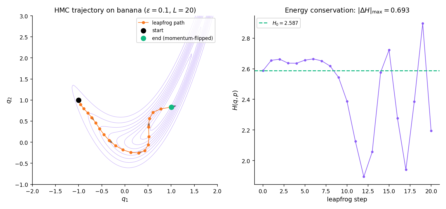
Target . Gradient is smooth and cheap to evaluate. Run HMC with , , mass matrix . Starting from , HMC flows along the banana ridge — a single trajectory can traverse from one end to the other, whereas random-walk Metropolis with any reasonable scale needs thousands of steps for the same distance. The acceptance rate comfortably exceeds 0.6 under these settings; the 0.234 / 0.44 random-walk rule does not apply.
Symplectic integrators conserve a modified Hamiltonian exactly, so while oscillates by per step, the oscillation stays bounded as grows. Non-symplectic methods (e.g., Runge–Kutta applied to Hamilton’s equations) suffer energy drift that grows linearly with — the chain would reject almost every proposal at long horizons. NEA2011 §5.4 derives the leapfrog modified Hamiltonian in full.
Standard HMC practice targets acceptance 0.65–0.85 — higher than random-walk’s 0.234 / 0.44 because HMC proposals are near-deterministic and should land close in energy. Too-low acceptance signals is too large (energy drift swamps the target density); too-high acceptance signals is too small (we’re under-exploring). Divergences — iterations where exceeds a threshold — indicate leapfrog has “fallen off” the energy manifold; in Stan / PyMC these are reported and usually signal a reparameterization opportunity.
The mass matrix defines the momentum distribution and hence the geometry HMC sees. The theoretically motivated choice is — Fisher information at the posterior mode — because then the transformed target is locally standard Normal and HMC’s Gaussian-momentum default is well-conditioned. This connects to Topic 14 Theorem 4 (MLE asymptotic normality; the posterior is approximately Gaussian with covariance at large ) and to Topic 25 §25.8’s Remark 16 Laplace-at-MAP approximation, which provides the standard HMC warm-start in practice: initialize at and set from the Laplace Hessian.
Curved ridge — HMC flows along curvature where RWM rejects. Featured-figure geometry (§26.4 Fig 4). Click anywhere on the main panel to reset the starting position.
26.5 The No-U-Turn Sampler
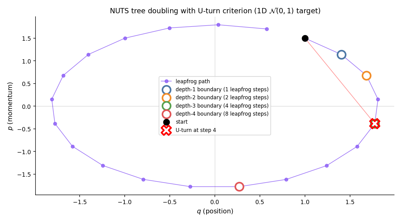
HMC’s two tuning parameters — leapfrog step size and trajectory length — are hard to pick by hand. Too-small under-explores; too-large wastes computation on trajectories that fold back on themselves. The No-U-Turn Sampler (NUTS, Hoffman–Gelman 2014) solves the length problem adaptively: extend the trajectory by binary doubling until the endpoints would turn back toward each other, then terminate. Combined with dual-averaging step-size adaptation during warmup, NUTS has no user-tunable hyperparameters — the pedagogical reason Stan and PyMC ship it as the default.
Given forward and backward trajectory endpoints and (with initially), a U-turn is detected when either of
holds. Intuitively: the trajectory has turned far enough that its endpoint momenta no longer point outward along the displacement vector. NUTS terminates doubling when a U-turn is detected on any subtree.
The NUTS sampler with dual-averaging step-size adaptation and slice-sampling-based subtree validity preserves on the extended state space .
Proof is not reproduced here; see HOF2014 Theorem 1 for the slice-sampling + multinomial-sampling argument. The key ingredients are (i) the slice variable ensures subtree nodes are valid samples from the typical set, (ii) uniform sampling from the valid subtree preserves by a deferred MH correction, and (iii) the U-turn stopping rule is reversible — terminating at a U-turn gives the same distribution whether we build forward or backward. HOF2014 Algorithms 2–3 state the recursive tree-doubling; Algorithm 6 gives the production-quality weighted-multinomial sampling scheme.
The canonical NUTS stress test is Rubin’s 1981 8-schools hierarchical model (GEL2013 §5.5). Eight observed treatment effects with school-level effects and hyperpriors on . At small , the posterior develops Neal’s funnel — a narrow neck where concentrates near zero. NUTS with Stan’s default settings handles this acceptably; non-centered reparameterization (§26.8 Rem 23, Topic 28) improves mixing further. Full applied workflow in §26.9 Example 11.
During a warmup phase (~1000 iterations), NUTS runs a dual-averaging scheme that targets acceptance around 0.8 by adjusting on the fly (HOF2014 §3.2). After warmup, is frozen and sampling begins. The adaptation is optimization-free — just Robbins–Monro stochastic approximation on the acceptance deviation — and converges reliably under Hoffman–Gelman’s conditions.
Stan (since 2014), PyMC (since 2016), and NumPyro all ship NUTS as their default sampler. The practical implication for practitioners: specify the model in the DSL, let NUTS sample, check and ESS. The §26.9 workflow assumes this; implementation internals are deferred to formalML: Probabilistic Programming (§26.10 Rem 33).
26.6 Convergence diagnostics
Every MCMC algorithm preserves its target asymptotically. The practical question is whether a finite-length chain has run long enough to represent the target — and since MCMC samples are dependent, standard iid intuitions about sample size don’t apply. Two diagnostics dominate applied work: Gelman–Rubin (has this chain mixed across its starting region?) and effective sample size (how many iid-equivalent samples does this correlated chain represent?).
Suppose we run chains of length from dispersed starting points, on a scalar summary of the chain state. Let and be the -th chain’s sample mean and (unbiased) sample variance, and the grand mean across chains. Define
The Gelman–Rubin statistic is
When chains have converged to , the between-chain variance falls to the within-chain variance and . Stan’s default threshold is before declaring convergence. detects non-convergence — high means chains disagree — but does not prove convergence; see §26.8 Rem 22 and the stuck-chain failure mode.
For a single chain of length with lag- autocorrelation , the effective sample size is
In practice the infinite sum is truncated by Geyer’s initial-positive-sequence estimator: group consecutive lags into pairs , accumulate until the first non-positive pair, and stop. For AR(1) with parameter , the theoretical , so gives and .
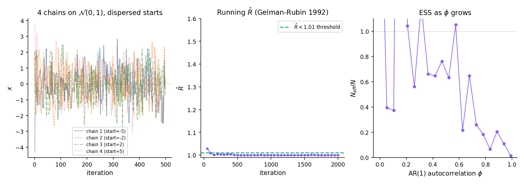
Initialize four chains at positions targeting with a random-walk Metropolis proposal at the RGG-1997 optimum. At iteration 100, chains are still concentrated near their starts — signals mixing has not occurred. By iteration 2000, chains have interpenetrated; has dropped below 1.01. The dashboard component below lets you scrub through this collapse interactively.
Generate an AR(1) chain with iid. This has stationary variance 1, but lag-1 autocorrelation . For samples at , the Geyer-IPS estimator gives — the 5000 correlated samples carry the information of roughly 263 iid samples. At , falls below 1%.
A low and a high ESS are necessary but not sufficient for convergence — chains that have collectively missed a mode show despite the posterior being fundamentally wrong (§26.8 Ex 10). ROB2004 Ch. 12 is forceful on this point: diagnostics tell us when the sampler has failed, not when it has succeeded. Substantive prior knowledge — does the posterior make sense? are credible intervals plausible? — remains the primary convergence check.
Vehtari et al. 2021 (“Rank-normalized split- and improved ESS”) updates to address two GEL1992 weaknesses: (i) sensitivity to marginal non-normality (addressed via rank-normalization), and (ii) insensitivity to intra-chain drift (addressed by splitting each chain in half and treating the halves as separate chains). Stan 2.21+ and PyMC 5+ use this variant. The GEL1992 formulation in Def 6 is still the pedagogical anchor.
Stan’s defaults: per parameter and per parameter before the chain is considered safe to report. The guidance comes from Monte Carlo standard error: at , the 95% MC-CI half-width is — less than 10% of the posterior standard deviation, which is typically the target precision for downstream inference.
Dispersed starts collapse onto the mode within ~200 iter. R̂ drops from ≈ 1.3 → < 1.01 — the happy path.
26.7 The ergodic theorem and MCMC-CLT
MCMC is justified by a dependent-sequence analog of the Strong Law of Large Numbers. Where Topic 10 Theorem 10.5 (Kolmogorov/Etemadi) guarantees that iid sample means converge almost surely to the expectation, the Markov-chain ergodic theorem extends the same conclusion to time averages along a chain — provided the chain is irreducible, aperiodic, and positive recurrent.
Let be a Markov chain on state space with transition kernel and invariant distribution . Assume:
- π-irreducibility. For every with and every , there exists with .
- Aperiodicity. for some (hence all) in the support.
- Positive recurrence. for every with , where is the first return time to .
Then for every ,
Equivalently: time averages converge to almost surely. This generalizes Topic 10 Thm 10.5 (iid SLLN) to dependent sequences; the new ingredients are irreducibility, aperiodicity, and positive recurrence replacing iid independence.
Proof 4 Proof of Thm 5 (ergodic theorem, sketch) [show]
Step 1 — reduction to regeneration. Under π-irreducibility + aperiodicity + positive recurrence the chain is positive Harris recurrent. These conditions give a small set and a minorization: there exist , integer , and a probability measure with
Athreya–Ney splitting constructs an auxiliary binary variable: whenever the chain enters , trigger a “regeneration” with probability , drawing the next state from and forgetting history. Regeneration times partition the chain into iid blocks.
Step 2 — block sums are iid. Define
By regeneration, is iid. The Kac formula gives
Positive recurrence ⇒ .
Step 3 — apply Topic 10 Thm 10.5 to the block sums. The are iid with . By the Kolmogorov/Etemadi SLLN (Topic 10 Thm 10.5),
This is the canonical bridge: time averages converge to almost surely. This generalizes Topic 10 Thm 10.5 (iid SLLN) to dependent sequences; the new ingredients are irreducibility, aperiodicity, and positive recurrence replacing iid independence.
Step 4 — renewal interpolation. Let count regenerations by time . Elementary renewal theory: almost surely. Then
with absorbing the partial last block.
Step 5 — bridge made explicit. The iid SLLN operates on the block sums , not directly on . Regeneration structure — induced by (i) irreducibility (ensures is reached), (ii) aperiodicity (permits Athreya–Ney minorization), (iii) positive recurrence (makes ) — converts the correlated chain into an iid-of-blocks sequence. The three conditions are the additional ingredients the Markov extension requires beyond iid independence.
∎ — sketch, using Topic 10 Thm 10.5 (Kolmogorov/Etemadi SLLN) for the block-sum SLLN, Athreya–Ney splitting (MEY2009 §5.1), and the renewal theorem (MEY2009 §17.1). Full proof: MEY2009 Thm 17.0.1.
Under geometric ergodicity (a strengthening of positive recurrence requiring exponential return times), for with suitable regularity,
with asymptotic variance
Proof is not reproduced; see VDV1998 §2 for the general martingale-CLT machinery and Kipnis–Varadhan 1986 for the Markov-chain specialization under geometric ergodicity conditions. The key structural difference from the iid CLT: the asymptotic variance picks up autocovariance terms — the reason ESS (§26.6 Def 7) is less than the chain length. The Monte Carlo standard error is , consistent with the ESS interpretation as an effective count of iid-equivalent samples.
Estimating from a single chain is the practical MCMC analog of estimating population variance. The batch-means estimator (Jones et al. 2006) splits the chain into batches of size , computes per-batch means , and sets
For iid samples from , this estimator converges to the variance 1. For AR(1) with , it inflates to approximately , matching the theoretical .
![Two-panel ergodic-theorem figure. Left: running mean of four chains on the standard Normal target, all converging to E_π[f] = 0 as iteration grows — the almost-sure convergence guaranteed by Thm 5. Right: the √n-scaled error √n(bar f_n - 0) collected across 500 independent runs, plotted as a histogram overlaid with the N(0, σ²_MC) MCMC-CLT reference curve (σ²_MC estimated via batch means).](/images/topics/bayesian-computation-and-mcmc/26-7-ergodic-running-mean.png)
The ergodic theorem is the bridge from Topic 10 to modern computational statistics. Time averages converge to almost surely. This generalizes Topic 10 Thm 10.5 (iid SLLN) to dependent sequences; the new ingredients are irreducibility, aperiodicity, and positive recurrence replacing iid independence. Roughly: iid independence is a very strong form of “the past stops mattering”; under the ergodic conditions, the past stops mattering after a random — but finite-on-average — recurrence time.
MCMC-CLT gives the applied MC standard error , where is the effective sample size (§26.6 Def 7). The practical workflow: run a chain, estimate via batch means, report — the exact same construction as frequentist CIs, with in place of .
26.8 Failure modes
The ergodic-theorem conditions are not automatic — bimodal posteriors can trap chains in a single mode indefinitely, polynomial tails can destroy geometric ergodicity, and bad starting points can leave chains stuck for the entire computational budget. The diagnostics of §26.6 detect some of these; the rest require substantive knowledge of the posterior.
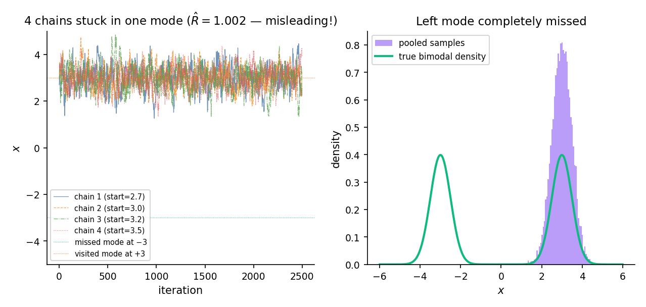
Consider the mixture . Both modes have probability 1/2; the valley between them has density ~, effectively zero at double precision. Run four random-walk Metropolis chains starting at with a local proposal scale of 0.5. The chains centered at stay there; the chains centered at stay there. Neither group ever visits the other mode within the 5000-iteration budget.
The between-chain variance is large (chains have different means — one pair near , one near ), but so is the within-chain variance — because “variance around the local chain mean” is dominated by the motion within each mode. When we compute , the ratio is not catastrophically large, and comes out near 1.0 despite the pooled posterior missing the valley entirely. The diagnostic is fooled.
This is the canonical caution in §26.6 Rem 16: low is not a proof of convergence. Multi-modal problems require domain knowledge (is the posterior expected to be multi-modal? if so, tempering or dispersed restarts are mandatory).
Geometric ergodicity fails when the target has polynomial tails and the proposal is light-tailed: returns to typical-set sets take polynomial (not exponential) time, the Kipnis–Varadhan CLT conditions fail, and batch-means variance estimates become unreliable. ROB2004 §7.3 gives conditions for geometric ergodicity of random-walk Metropolis; the standard fix for heavy-tailed targets is a Student- proposal (polynomial tails match polynomial tails) or a reparameterization that mod-transforms the tail behavior. Roberts–Rosenthal 2004 Thm 13 is the general geometric-ergodicity statement.
Single-chain MCMC is diagnostically weak: any pathology that affects the chain uniformly (stuck in a mode, never reaching the typical set, divergent leapfrog trajectory) can look fine from inside. Multi-chain MCMC with dispersed starting points — standard practice since GEL1992 — lets detect disagreement between chains that started in different regions. The canonical heuristic: initialize chains by sampling from an over-dispersed approximation to the posterior, typically 4 chains with starting points at the MAP 3 MAP-std in each coordinate.
Hierarchical models produce Neal’s funnel: the hyperparameter (group-level scale) is inversely correlated with the conditional standard deviation of the individual-level effects , producing a long thin neck where concentrates near zero. HMC trajectories in this region either diverge (energy explodes) or crawl along the narrow direction. The standard mitigation is non-centered reparameterization: sample and set , decoupling the funnel’s correlation structure. NEA2011 §4 and Topic 28 develop this in the hierarchical-model context.
26.9 Applied workflow: the 8-schools hierarchical model
Putting it all together: Rubin 1981 / GEL2013 §5.5 eight-schools model is the canonical hierarchical-Bayes demonstration. Eight observed treatment effects from an educational intervention, each with a standard error. The question: is the “true” effect shared across schools, completely independent, or partially pooled?
Data:
Model:
The workflow: specify the model in Stan or PyMC, let NUTS sample 4 chains × 2000 iterations with 1000 warmup each, inspect and ESS for every parameter, plot the posterior for (this is where Neal’s funnel lives) and for each (partial pooling visible: school 1’s raw shrinks substantially toward the group mean ).
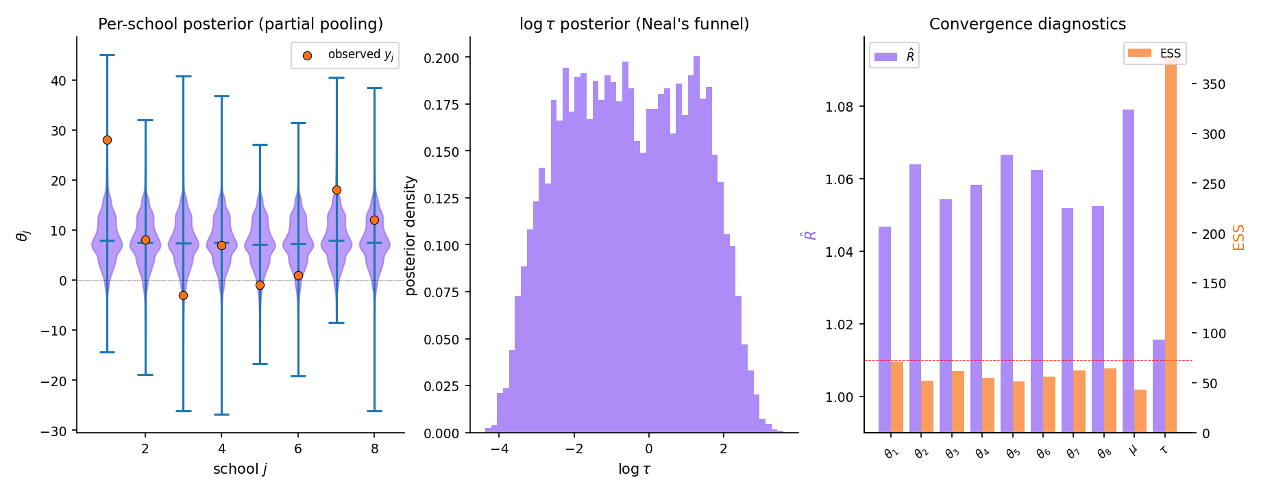
Running the 8-schools model in Stan with default settings — 4 chains, 2000 post-warmup iterations each — produces for every parameter and for every parameter. Neal’s funnel is visible in : the posterior concentrates in a narrow neck near that fans out as grows. The school-level effects all shrink toward the group mean ; the shrinkage is stronger for schools with larger observational (less individual information). The partial-pooling posterior has noticeably smaller uncertainty than either fully-pooled ( for all , 1 parameter) or no-pooling ( with known , 8 independent problems) analyses. This is the classical Bayesian hierarchical advantage, made computational by NUTS.
The non-centered reparameterization — sample and set — eliminates the funnel at the cost of slightly more verbose model code. Full treatment in Topic 28.
Note on implementation: the notebook backing this topic uses conjugate Gibbs with an Inverse-Gamma prior on for self-containment and speed; production workflows use NUTS with a Half-Cauchy prior on per Gelman 2006 (“Prior distributions for variance parameters in hierarchical models”). The two yield comparable posteriors but differ on the marginal — the Half-Cauchy is the applied-recommendation default.
26.10 Forward map
Topic 26 covers the core four algorithms and their diagnostics. Ten specialized methods — each a coherent research area in its own right — defer to downstream topics or to formalML: formalml.com . Two in-Track-7 topics extend the Bayesian framework further. One cross-track connection to variational inference frames the speed-exactness trade-off.
Topic 27 develops Bayes-factor-based model comparison and Bayesian model averaging (BMA). The computational core is estimating marginal likelihoods from MCMC draws — hard because MCMC only gives the posterior’s shape, not its normalization. Standard methods: bridge sampling (Meng–Wong 1996), path sampling via thermodynamic integration, nested sampling (Skilling 2006). The Topic 24 BIC-Laplace approximation is the low-effort first pass; Topic 27 gives the high-effort production versions.
Topic 28 generalizes the 8-schools example to arbitrary hierarchical models. The computational pattern is Gibbs (when conjugate) or NUTS (when not); the scientific content is partial pooling, shrinkage, and empirical Bayes as degenerate limits of full hierarchical inference. Continuous shrinkage priors (horseshoe, Cauchy+) complete the modern applied toolkit.
When conjugacy fails and MCMC is too slow (hierarchical models with millions of parameters, deep Bayesian neural networks), variational inference approximates the posterior with a tractable family by minimizing . VI is orders of magnitude faster than MCMC for large ; MCMC is asymptotically exact, VI is not. Both are supported in Stan, PyMC, and NumPyro; the practical rule is “start with VI for fast exploration, switch to MCMC for final inference.” Full treatment at formalML: Variational Inference .
Adaptive MCMC — Haario–Saksman–Tamminen 2001, Roberts–Rosenthal 2009 — updates the proposal covariance during the run using the empirical covariance of accumulated samples. Requires diminishing-adaptation conditions (the adaptation must eventually stop) to preserve ergodicity; practical implementations freeze the adaptation after a warmup phase. BRO2011 Ch. 4 is the standard reference.
Reversible-jump MCMC (Green 1995) generalizes MH to trans-dimensional state spaces — models whose dimension is itself a parameter (variable selection, mixture models with unknown component count). The dimension-changing moves require Jacobian corrections to the acceptance ratio. BRO2011 Ch. 3 gives a clean exposition; formalML: Reversible-Jump MCMC develops the formalml treatment.
Riemann-manifold HMC (Girolami–Calderhead 2011) replaces HMC’s constant mass matrix with a position-dependent metric — Fisher information evaluated at the current position. Pays local geometry respect; requires second-derivative computation of . formalML: Riemann-Manifold HMC develops the differential-geometry machinery.
Stochastic-gradient Langevin dynamics (Welling–Teh 2011) and SGHMC (Chen–Fox–Guestrin 2014) replace the full-batch gradient in HMC / Langevin with a mini-batch gradient plus injected noise, scaling MCMC to large- datasets at the cost of introducing asymptotic bias. Standard in Bayesian deep learning. formalML: Stochastic-Gradient MCMC develops the theory.
Sequential Monte Carlo / particle filters target a sequence indexed by time or annealing parameter, importance-sampling from and resampling. The natural framework for state-space models (Kalman filter generalizations) and rare-event estimation. Parallel to MCMC’s single-target framework. formalML: Sequential Monte Carlo .
Parallel tempering / simulated tempering runs multiple chains at different temperatures (target ); chains occasionally swap states via an MH-style accept step. Hot chains explore freely; cool chains sample precisely; swaps transfer the hot-chain exploration to cool-chain precision. Standard multi-modal mitigation. BRO2011 Ch. 11.
Modern Bayesian practice runs through probabilistic programming languages (PPLs): Stan, PyMC, NumPyro, Turing.jl. Users specify a model in a DSL; the compiler generates the log-density and its gradient (automatic differentiation), then hands the result to NUTS. Compiler engineering — transformation to unconstrained space, reverse-mode autodiff, target densification — is outside Topic 26’s scope. formalML: Probabilistic Programming .
Nested sampling (Skilling 2006) transforms the marginal-likelihood integral into a 1-D integral over the prior’s likelihood levels, sampled via a sequence of constrained-prior draws. Natural for problems where the marginal likelihood itself is the target (Bayes factors, cosmological model comparison). Topic 27 develops the modern machinery.
Bayesian nonparametrics — Chinese restaurant process / Dirichlet process mixtures, Indian buffet process — extends Bayesian inference to infinite-dimensional parameter spaces. MCMC for these models involves custom samplers (slice sampling, truncation, finite-dimensional approximations) tied to the specific construction. formalML: Bayesian Nonparametrics .
Slice sampling (Neal 2003) is an auxiliary-variable MH variant that avoids proposal-scale tuning: introduce a uniform-height auxiliary variable below the density, then draw uniformly over the level set . Adaptive without dual-averaging; robust on 1-D problems. Often described as “MH-without-tuning.” Less used than HMC / NUTS at scale because the level-set sampling is expensive in high dimensions.
Topic 26 closes Track 7’s computational pass. The remaining two Track 7 topics — Topic 27 on Bayesian model comparison and BMA, Topic 28 on hierarchical Bayes — build on Topic 26’s MCMC machinery to handle model uncertainty and group-structured priors, respectively. The ergodic-theorem bridge to Topic 10 is the theoretical anchor: MCMC’s asymptotic contract is a dependent-sequence SLLN, and every diagnostic and variance estimator we compute traces back to the Kipnis–Varadhan CLT.
References
- Nicholas Metropolis, Arianna W. Rosenbluth, Marshall N. Rosenbluth, Augusta H. Teller & Edward Teller. (1953). Equation of State Calculations by Fast Computing Machines. Journal of Chemical Physics, 21(6), 1087–1092.
- W. K. Hastings. (1970). Monte Carlo sampling methods using Markov chains and their applications. Biometrika, 57(1), 97–109.
- Stuart Geman & Donald Geman. (1984). Stochastic Relaxation, Gibbs Distributions, and the Bayesian Restoration of Images. IEEE Transactions on Pattern Analysis and Machine Intelligence, 6(6), 721–741.
- Radford M. Neal. (2011). MCMC using Hamiltonian dynamics. In Handbook of Markov Chain Monte Carlo, Chapter 5. CRC Press.
- Matthew D. Hoffman & Andrew Gelman. (2014). The No-U-Turn Sampler: Adaptively Setting Path Lengths in Hamiltonian Monte Carlo. Journal of Machine Learning Research, 15(47), 1593–1623.
- Andrew Gelman & Donald B. Rubin. (1992). Inference from Iterative Simulation Using Multiple Sequences. Statistical Science, 7(4), 457–472.
- Sean P. Meyn & Richard L. Tweedie. (2009). Markov Chains and Stochastic Stability (2nd ed.). Cambridge University Press.
- Christian P. Robert & George Casella. (2004). Monte Carlo Statistical Methods (2nd ed.). Springer.
- Steve Brooks, Andrew Gelman, Galin L. Jones & Xiao-Li Meng (Editors). (2011). Handbook of Markov Chain Monte Carlo. CRC Press.
- Andrew Gelman, John B. Carlin, Hal S. Stern, David B. Dunson, Aki Vehtari & Donald B. Rubin. (2013). Bayesian Data Analysis (3rd ed.). CRC Press.
- A. W. van der Vaart. (1998). Asymptotic Statistics. Cambridge University Press.