Regularization & Penalized Estimation
When OLS and IRLS break under collinearity or separation, a penalty term on the loss restores well-posedness. Ridge gives MSE-improvement (Hoerl–Kennard 1970); lasso gives variable selection through soft-thresholding (Tibshirani 1996); elastic net combines them; coordinate descent (Tseng 2001) is the algorithmic engine, and cross-validation picks the penalty parameter.
23.1 When OLS and IRLS fail: collinearity and separation
Topic 21 built the OLS framework on a single working assumption: is invertible. Topic 22 extended this to for IRLS. Both assumptions fail in production. The canonical failure modes are multicollinearity (predictors so correlated that ) and separation (a logistic-regression hyperplane that perfectly classifies the training data, sending ). Both pathologies have one fix in common: add a penalty term that grows with , making the penalized objective coercive even when the unpenalized one is not.
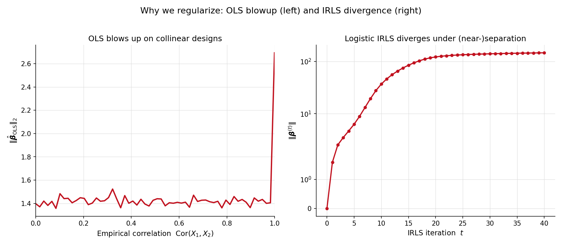
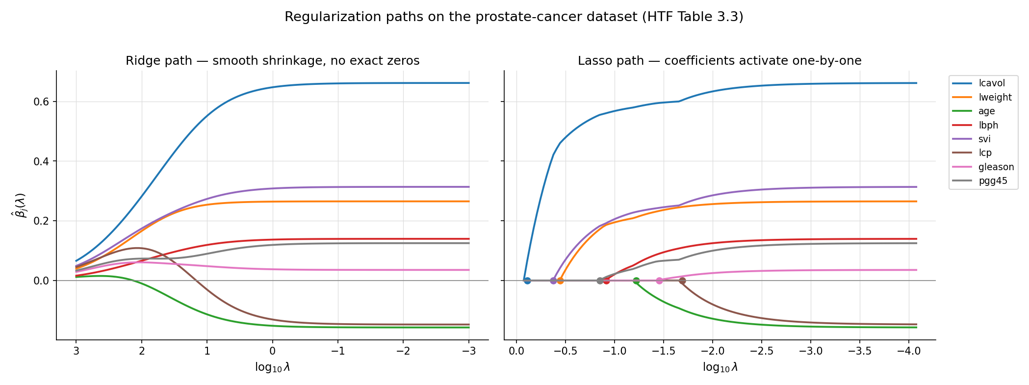
The prostate-cancer dataset (HTF Table 3.3, used as the running benchmark throughout this topic) has 97 patients and 8 predictors. Two of those predictors — lcavol (log cancer volume) and lcp (log capsular penetration) — are tightly correlated (). If we artificially amplify that correlation by replacing lcp with for , the OLS coefficient vector does not just become unstable — it diverges. The figure below tracks as a function of the artificial correlation strength: by the L²-norm has grown by three orders of magnitude. Individual coefficients on lcavol and lcp swing in opposite directions, fitting noise.
This is the §21.5 multicollinearity warning made concrete. The variance inflation factor (VIF) flags it; ridge regression fixes it. The cure works by adding to the objective: the closed form is well-defined as long as , no matter how singular becomes.
Topic 22 §22.4 Rem 8 flagged separation as the second canonical pathology: when a hyperplane in predictor space perfectly classifies the binary response, the logistic log-likelihood is monotone-increasing along the direction , and IRLS iterates run away to . The brief promised the fix would arrive in Topic 23. Here it is.
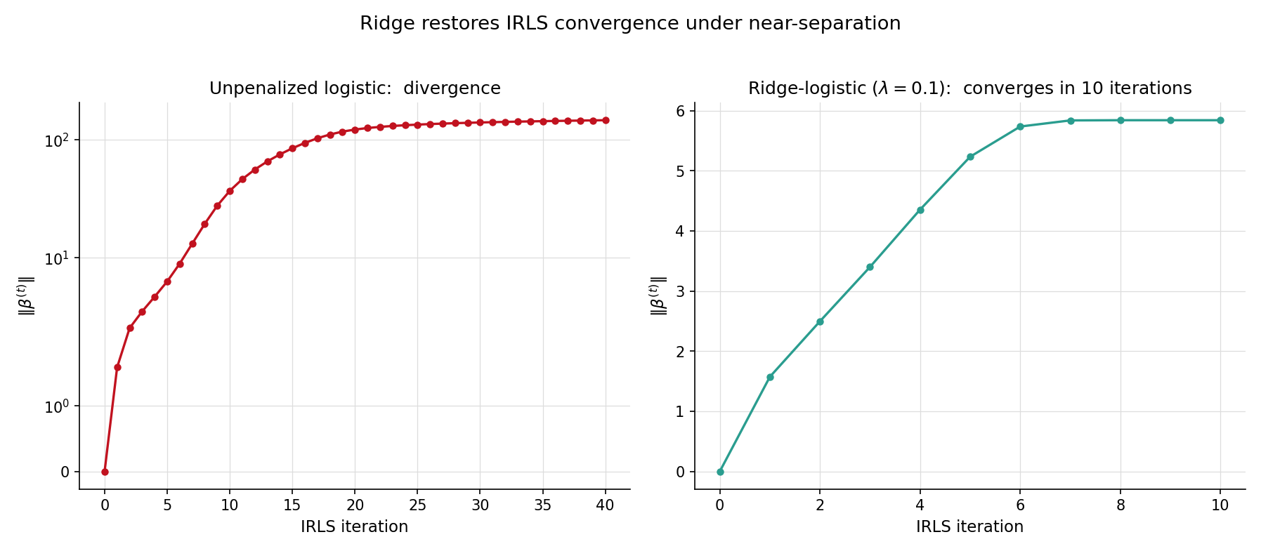
The EXAMPLE_10_GLM_DATA preset (n = 120, p = 2) is a near-separation problem: the two classes are almost linearly separable, with only a handful of overlap points. Bare glmFit from Topic 22 reports converged = false after the maximum iteration count — by iteration 50, has crossed 100 and is still growing. Adding a ridge penalty with changes the picture immediately: convergence in around 10 outer iterations to a finite, well-determined estimate. The §23.6 Ex 8 worked example develops this in detail, but the punchline lands here in §23.1: regularization is not just a remedy for the squared-error case — it restores well-posedness for IRLS too.
Penalized estimation is older than computer-era statistics. Tikhonov 1943 introduced for integral-equation regularization in physics — 27 years before its statistical rediscovery. Hoerl & Kennard 1970 put ridge on the statistical map with the MSE-improvement theorem (§23.3 Thm 1) and the ridge-trace diagnostic. Tibshirani 1996 introduced the lasso, replacing with to obtain variable selection — a paper that has accumulated more than 40,000 citations. Firth 1993 had earlier introduced a Jeffreys-prior penalty as a separation cure for logistic regression; it is one of two practical answers to the §23.1 Ex 2 pathology, with ridge being the other (§23.6 Rem 11). The unifying framework — penalty as additive term on the negative log-likelihood — is what we develop next.
23.2 The penalized-objective framework
Notation (extending §21.4 and §22.2). Throughout Topic 23, is the penalty parameter and is a convex penalty function ( for ridge, for lasso, for elastic net). The soft-thresholding operator is , applied componentwise to vectors. The active set is . The partial score at coordinate is . We write for the data-generating “true” coefficient and for the regularization path.
The ridge regression estimator at penalty parameter is
The closed form, derivable by setting the gradient to zero, is
The matrix is positive-definite for any , so the estimator exists and is unique even when is rank-deficient — the regression.ts ridgeFit implements exactly this closed form via Cholesky on the augmented Gram matrix. The scaling on the penalty matches the lasso convention below ( on residuals throughout) and lines up with sklearn.linear_model.Ridge(alpha=λ) directly: alpha = λ gives identical fits.
The lasso estimator at penalty parameter is
The regression.ts lassoFit adopts this convention (no on residuals); to get the same fit out of sklearn.linear_model.Lasso(alpha) — whose objective is — call it with alpha = λ/n. There is no closed form in general; coordinate descent (§23.4) is the standard solver. Unlike ridge, the lasso produces exact zeros in — the variable-selection property, established formally in Thm 2 below.
For a general log-likelihood and a convex penalty , the penalized maximum-likelihood estimator is
This is the unifying framework: ridge is the squared-error special case with ; lasso is ; penalized GLMs (§23.6) replace with the GLM negative log-likelihood. The Bayesian reading via §23.7 Thm 5 is that is the negative log-prior, making penalized MLE identical to MAP estimation.
Setting :
Rearranging,
The Hessian is positive-definite for , so the stationary point is the unique global minimum. Compare to OLS (Topic 21 §21.4 Thm 3): the only difference is the term added to the diagonal. Geometrically, ridge replaces an ill-conditioned matrix with a well-conditioned one by inflating its smallest eigenvalues from near-zero up to at least .
Both ridge and lasso are not scale-equivariant: rescaling a predictor changes its penalty contribution. If is measured in centimeters, its coefficient is 100× the value it would be in meters; the lasso would shrink the centimeter-scale coefficient harder. Standard practice is to standardize predictors before fitting — center each at zero and scale to unit variance. The intercept is then absorbed by centering , and the recovered coefficients are converted back to original units after the fit. The regression.ts implementation does this by default (standardize: true).
This standardization preserves the geometric clarity of the penalty (every coefficient sits on the same scale) at the cost of breaking equivariance under reparameterization — the price of a penalty that ignores the model’s sufficient statistic structure (Topic 16 §16.4). For genuine equivariance, one would need a scale-invariant penalty like , which is rarely used in practice.
Standard convention — adopted by glmnet, sklearn, and regression.ts — is to leave the intercept unpenalized. The intuition: shifting all predictors by a constant should not change the model, but it would change the intercept; penalizing the intercept would couple the model to the location of the predictors. Mechanically, after centering and standardizing , the intercept becomes and is recovered post-fit as . The penalty applies only to the slope coefficients .
Write with the singular values. The ridge fit can be written
OLS is the case: . Ridge replaces with — a smooth shrinkage that hits hardest where is small (the directions of low data variance). Lasso is non-uniform: its shrinkage acts in the original predictor coordinates, not the SVD coordinates, and produces exact zeros rather than smooth shrinkage. The two penalties differ both in what they shrink and how.
23.3 Featured: ridge MSE-improvement and lasso KKT
Topic 22’s §22.3 paired two featured theorems — the canonical-link score identity and IRLS = Fisher scoring = Newton — and earned its place in the topic’s structure as the load-bearing block. §23.3 mirrors that structure with two of its own.
Let be the true coefficient vector under the fixed-design Normal linear model with and of full column rank. Then there exists such that for every coordinate ,
The total MSE is strictly smaller at than at .
Proof 1 Ridge MSE-improvement (Hoerl–Kennard 1970) [show]
Setup. Fix , , and a full-column-rank design . Let , so that and . At , and we recover OLS: unbiased, with variance .
Total MSE decomposition. Writing ,
SVD coordinates. Write with , . In the rotated coordinates (so ), the MSE decomposes coordinatewise:
First-order Taylor at . Expanding each summand (holding fixed):
- Squared-bias contribution: — at small .
- Variance contribution: — at small with negative coefficient.
Derivative at . Summing over :
Because the derivative is strictly negative at and is continuous (indeed smooth) in , there exists with .
Component-wise strengthening. The same argument applied to each diagonal entry of the MSE matrix shows that every component is strictly smaller than at some . Taking gives uniform strict improvement. ∎ — using the SVD decomposition of (Topic 8 §8.5) and the MSE = bias² + variance decomposition (Topic 13 §13.2).
The sign of the first-derivative term is the entire argument: variance shrinks linearly in while bias grows quadratically, so for small variance wins. The bias-variance tradeoff is not a vague principle but a precise inequality. The catch: depends on the unknown and — in practice, cross-validation (§23.8) picks it.
Let . Define the partial score . The KKT optimality conditions are
For orthonormal designs , the solution has the closed form
where is the soft-thresholding operator.
Proof 2 Lasso KKT characterization + soft-thresholding (Tibshirani 1996) [show]
Setup. Let . The first term is convex and differentiable; the second is convex but non-differentiable at any . The global minimum exists (the objective is coercive and continuous) and is characterized by the subgradient optimality condition .
Subgradient of the L¹-norm. The subgradient of at is
Subgradient of . The gradient of the smooth part is . Hence
KKT conditions. Setting coordinatewise:
- If : .
- If : .
- If : , i.e., .
Active coordinates carry sign-matched score equal to ; inactive coordinates have partial score bounded by .
Orthonormal-design corollary. When , the partial score at simplifies to . Substituting into the KKT cases:
- : , valid when .
- : , valid when .
- : .
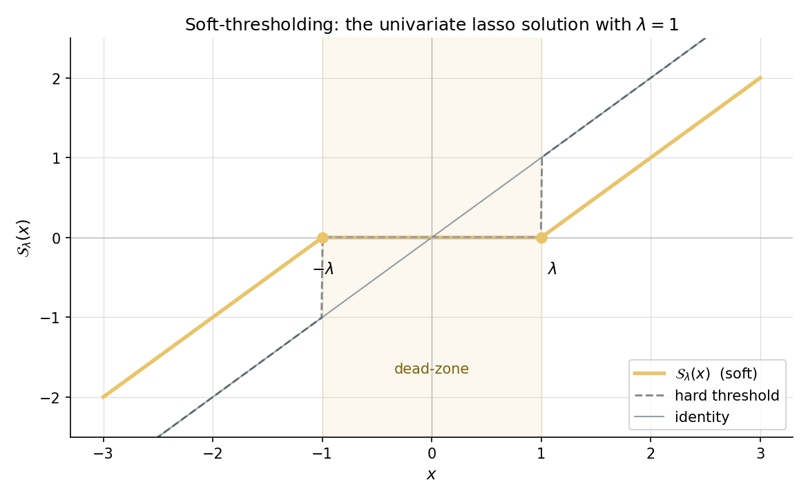
Soft-thresholding formula. The three cases collapse into
(Under the standardization convention used by lassoFit — column-centered with — this generalizes to on the partial residual; the algorithmic version is §23.4.) Every univariate coordinate-descent update for the lasso is one application of . ∎ — using subgradient calculus (formalCalculus: convex optimization).
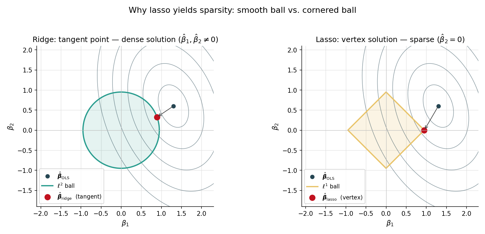
Step 4 is the headline result: the diamond-vs-circle picture in LevelSetExplorer literally shows active coordinates landing at on the diamond’s edge, and inactive coordinates landing at a vertex (where the L¹-ball is non-differentiable). The §23.4 coordinate-descent algorithm is one application of the orthogonal-design formula per coordinate per sweep, using the partial residual instead of directly.
Plugging the prostate-cancer design into the SVD-coordinate MSE formula from Proof 1, we can compute the bias² and variance contributions to total MSE as a function of . At (OLS), bias² is zero and variance carries all the weight. As grows, bias² rises quadratically while variance falls roughly proportionally to . The total MSE traces a U-shape with minimum somewhere in the middle. For the prostate dataset, that minimum lies near — large enough to substantially reduce variance on the small singular values, small enough to keep bias modest.
Take (so , scaling by for cleanness — for the canonical orthogonal-design corollary). Suppose . Then . Apply soft-thresholding at :
The third and fourth coordinates land in the dead zone and are zeroed out — this is variable selection in action. As grows, more coordinates fall into the dead zone; at the entire estimate is the zero vector. This is the geometric content of Thm 2’s orthogonal-design corollary made concrete.
Statistics courses introduce the bias-variance tradeoff with the equation and an exhortation to “find the right balance.” Thm 1 sharpens this to a precise mathematical statement: for any design and any nonzero true , some positive strictly beats OLS in total MSE — and component-wise, too. The tradeoff has a positive side: there is always free MSE on the table to be picked up by a small ridge penalty. The remaining question is how to find the right , which §23.8 answers.
The Hoerl–Kennard ridge MSE-improvement theorem has a 14-year-older sibling: Stein 1956’s inadmissibility result. For the multivariate Normal mean problem with , the natural estimator is inadmissible under squared-error loss — there exist estimators (the James–Stein shrinkage family) with strictly smaller risk for every . Ridge is a covariate-version of the same idea; the full Stein-identity proof is Topic 28 §28.5 Thm 2. The Lehmann–Romano admissibility framework (LEH2005 Ch. 5) shows that in the regression setting, ridge dominates OLS for specific ranges depending on and the design. The §23.7 Rem 17 returns to the Hodges-superefficiency tie-in flagged at Topic 14 §14.6 Rem 6.
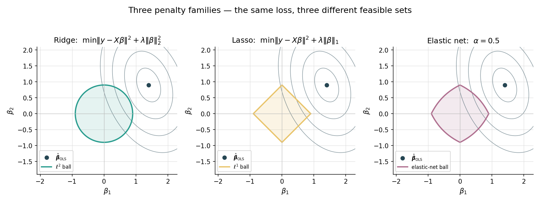
Both ridge and lasso can be re-cast as constrained optimization problems via Lagrangian duality:
- Ridge: subject to — minimize a quadratic on a Euclidean ball.
- Lasso: subject to — minimize a quadratic on an L¹ ball (a “diamond” in 2D, a cross-polytope in higher dimensions).
The OLS solution is the center of the elliptical contours of the quadratic loss. Ridge’s solution is the closest point on the Euclidean ball — a smooth shrinkage. Lasso’s solution is the closest point on the diamond — and because the diamond has corners precisely where one or more coordinates are zero, the closest point typically lands on a corner. Sparsity is the geometric consequence of the L¹ ball’s vertices. This is the picture the LevelSetExplorer makes interactive.
23.4 Coordinate descent and the glmnet algorithm
Ridge has a closed form. Lasso does not. The standard solver is cyclic coordinate descent — update one coordinate at a time, holding the others fixed, sweep through all coordinates, and repeat until convergence. Friedman, Hastie & Tibshirani’s glmnet paper (FRI2010) made this approach the production workhorse for penalized linear models and GLMs.
The active set of a coefficient vector is
For a lasso fit , is the selected variable set — the predictors the procedure judges worth keeping. As shrinks, grows; at , recovers OLS.
The cyclic-CD update for the lasso uses the soft-thresholding closed form (Thm 2’s orthogonal-design corollary) on the partial residual :
Standardization makes , so the denominator drops out and each coordinate update is one soft-thresholding step. A full sweep updates all coordinates; the algorithm terminates when the maximum coordinate change falls below a tolerance. With warm starts from a neighbouring , paths over a 100-point -grid are computed in essentially the time of one cold-start fit.
Let where is convex and continuously differentiable and each is convex (possibly non-differentiable). Assume is bounded below and coercive. Starting from and updating coordinate-by-coordinate as
the sequence converges to a global minimizer of . The lasso objective satisfies the hypothesis with and .
Proof 3 Cyclic coordinate descent convergence (Tseng 2001) [show]
Setup. as in the theorem, with convex and , each convex (possibly non-differentiable), and coercive. The cyclic-CD iterates are defined as in the theorem statement.
Monotone descent. Each univariate update can only decrease the objective, , with equality iff the previous already minimized the slice.
Boundedness of iterates. Because is coercive and the iterates are monotone-descending, the sublevel set is bounded. The sequence is therefore bounded and admits a convergent subsequence by Bolzano–Weierstrass.
Limit is a coordinatewise stationary point. By continuity of the univariate map (which holds because the slices are strictly convex — ‘s second partial in plus the convexity), the limit satisfies
for every . This is the coordinatewise stationarity condition.
Coordinatewise ⇒ global, via separability. Because with the non-smooth part separable (each depends on only one coordinate), the coordinatewise stationarity condition is equivalent to — and for convex , that is the global-minimum condition. The separability is essential: Tseng 2001 explicitly constructs counterexamples where cyclic CD on a non-separable non-smooth function fails to converge to the minimizer.
Full-sequence convergence. Because the slice-minima are unique (strict convexity per coordinate), every convergent subsequence of converges to the same global minimizer. By a standard sub-subsequence argument, the full sequence converges. ∎ — using Tseng 2001 Prop 5.1 and the lasso objective’s separable structure.
Step 5 is where the structural insight lives: coordinate descent works on the lasso because is a sum of single-coordinate functions. It would fail on the fused lasso (, used for piecewise-constant signals), which couples adjacent coordinates and breaks the separability. For non-separable non-smooth penalties, proximal-gradient methods (ISTA, FISTA) take over.
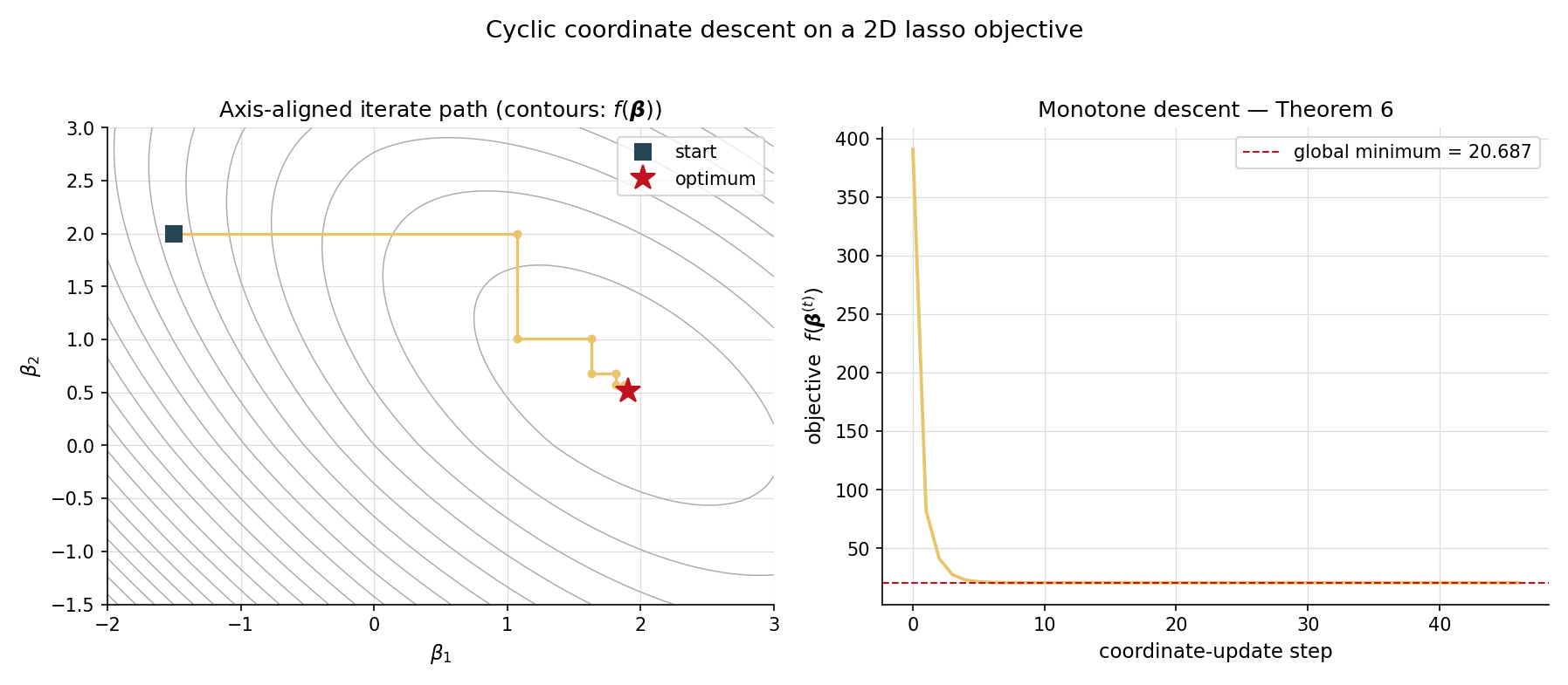
A two-coefficient lasso problem () lets us visualize the iterate path directly. With a small synthetic design and , the cold-start CD iterate trajectory makes a zigzag through coefficient space: each axis-aligned step minimizes one coordinate while holding the other fixed. The objective decreases monotonically (the right panel of the visualizer); the path converges to the global minimizer in around 47 coordinate updates (about 24 sweeps of 2 coordinates) at tolerance . With warm-start from the neighbouring , the same problem solves in 5–10 coordinate updates.
Before glmnet, the standard lasso solver was LARS (Least Angle Regression; Efron, Hastie, Johnstone & Tibshirani 2004). LARS computes the entire piecewise-linear regularization path exactly by tracking when each coordinate enters or leaves the active set as decreases. It is elegant — the path is piecewise linear — but slower in practice than coordinate descent for large , because each LARS step requires solving a linear system on the current active set. glmnet won out on engineering: cyclic CD is embarrassingly simple to vectorize, scales to in the millions, and supports any convex penalty (LARS is lasso-only). Topic 23 treats LARS as a historical pointer; for the algorithm itself, see HAS2009 §3.4.4.
A defining feature of glmnet is path computation with warm starts: instead of solving for one at a time from scratch, compute the path over a 100-point log-grid in one pass, using the solution at as the starting point for . Because consecutive values give nearby solutions, each warm-started fit needs only a few sweeps to converge — the per- cost drops by roughly an order of magnitude. The grid runs from (the smallest for which ) down to . The regularizationPath function in regression.ts implements this scheme.
For very large (gene-expression studies with predictors), even cyclic CD becomes a bottleneck. Two acceleration techniques are widely deployed: strong screening rules (Tibshirani et al. 2012) eliminate predictors that the KKT conditions guarantee will be inactive at the next , before any coord-descent updates — a – speedup. Proximal-gradient methods (ISTA, FISTA) take small gradient steps on the smooth part and apply soft-thresholding as the proximal operator; they generalize beyond separable non-smooth penalties (where coord descent fails) at the cost of slightly worse constants. regression.ts ships only the basic cyclic CD; production deployments should reach for glmnet or sklearn.linear_model.{Lasso, LassoCV} (also a CD implementation) with screening rules enabled.
23.5 Elastic net
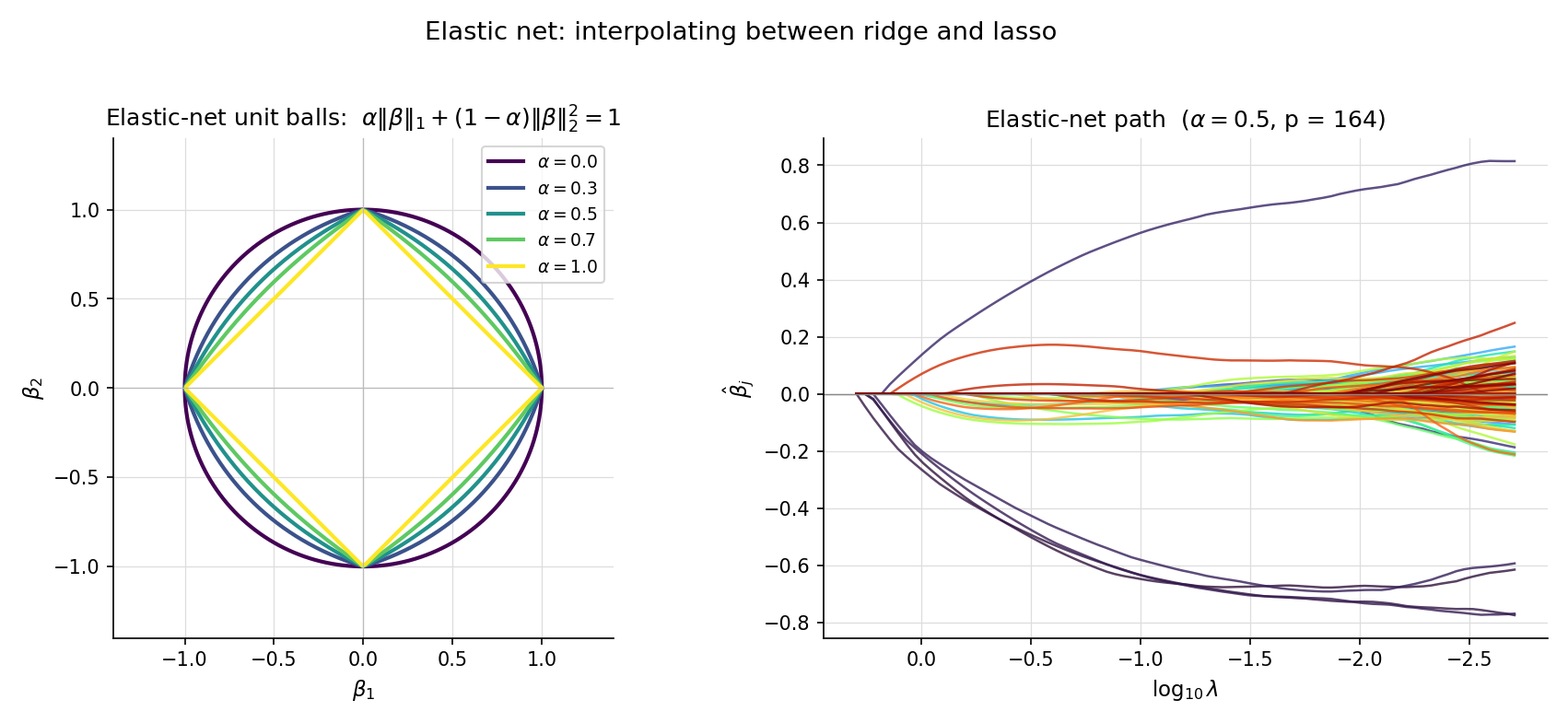
Lasso and ridge each have a failure mode. Lasso, on highly correlated predictors, tends to pick one and zero out its companions arbitrarily — a coin-flip choice that destabilizes interpretation across bootstrap samples. Ridge gives stable weight to all correlated predictors but never produces sparsity. The elastic net (Zou & Hastie 2005) interpolates: a convex combination of L¹ and L² penalties.
For and , the elastic-net penalty is
and the elastic-net objective is
recovers lasso (); recovers ridge with penalty — matching Def 1’s convention exactly. For , the penalty is strictly convex even when is rank-deficient — a property ridge has but lasso does not.
For any and , the elastic-net objective is strictly convex in , and the minimizer is unique — regardless of the rank of .
Brief argument: the Hessian of the smooth part is , which is positive-definite whenever . The L¹ term is convex (subdifferentiably), so the full objective is strictly convex. ZOU2005 Thm 1.
Take a synthetic problem with three pairs of perfectly correlated predictors plus four independent ones (the CORRELATED_FEATURES_DATA preset). The true coefficient is nonzero only at and — both members of correlated pairs. Lasso, run at the CV-optimal , picks one predictor from each correlated pair and zeros the other — and which one it picks varies arbitrarily across bootstrap samples. Elastic net with at the same effective penalty strength assigns nonzero weight to all four members of the correlated pairs, distributing weight across the group. The grouping effect: correlated predictors get similar coefficients, and the active set is more stable.
Zou & Hastie 2005 prove that for any two predictors and with (a strong correlation condition), the elastic-net coefficients satisfy
where is the correlation. As correlation , the bound forces — the coefficients are pulled together. For pure lasso (), the bound is vacuous (denominator zero), which is why lasso lacks the grouping effect.
Elastic net introduces a second hyperparameter, , on top of . Most production workflows fix a small grid of values (, say), run cross-validation to pick for each, and choose the combination with smallest CV error. The 2D grid is more expensive than the 1D lasso/ridge search but rarely prohibitively so. The figure shows the parameter plane on the prostate-cancer data, with CV-error contours and the optimal point marked.
23.6 Penalized GLMs
Topic 22’s IRLS framework extends to penalized GLMs essentially unchanged. Replace the negative log-likelihood with the penalized version, and the inner WLS step becomes a penalized WLS step.
For a GLM with log-likelihood (Topic 22 Def 3) and a convex penalty , the penalized-GLM estimator is
For ridge, ; for lasso, ; for elastic net, as in Def 5. The unpenalized intercept convention applies as usual.
Under a canonical link and a convex sub-differentiable penalty , the penalized-IRLS update at iteration solves
where and are Topic 22 Thm 2’s IRLS weights and adjusted response. For this is a ridge-WLS problem with closed form . For it is a weighted-lasso coord-descent inner pass.
Brief derivation: a second-order Taylor expansion of around produces the WLS quadratic surrogate exactly as in Topic 22 Proof 2; adding gives the penalized surrogate. Minimizing the surrogate is the next IRLS step. Convergence proceeds as in Tseng 2001 with the surrogate playing the role of .
The EXAMPLE_10_GLM_DATA preset (n = 120, p = 2) is the near-separation problem from §23.1 Ex 2. Topic 22’s bare glmFit reports converged = false after 50 iterations: has crossed 100 and is still growing. Calling penalizedGLMFit with family: 'binomial', link: 'logit', penalty: 'ridge', lambda: 0.1 instead converges in around 10 outer IRLS iterations to a finite estimate with — a small fraction of what the unpenalized fit would have produced. The ridge penalty makes the otherwise non-coercive objective coercive; the IRLS surrogate is then guaranteed to have a unique bounded minimizer at every step.
The Topic 22 EXAMPLE_6_GLM_DATA (credit-default logistic, n = 200, p = 2) becomes a high-dimensional problem when its predictors are expanded to degree 3 polynomials. The expanded design has p = 34 features (the CREDIT_DEFAULT_EXPANDED_DATA preset). Fitting a lasso-logistic at the CV-selected produces a sparse with around 6–10 active coefficients, automatically selecting the polynomial terms that contribute predictive signal. Pure logistic regression on the expanded design overfits badly; lasso-logistic regularizes both selection and shrinkage in one pass.
Ridge is one cure for logistic-regression separation; Firth’s penalized likelihood (FIR1993) is the other. Firth replaces the log-likelihood with where is the Fisher information — equivalent to a Jeffreys prior on . This penalty bounds the estimator without requiring a tuning parameter. In practice, Firth is the default in many epidemiology workflows where a single hyperparameter-free fix is preferred; ridge wins when cross-validation is feasible and the user wants explicit control over the bias-variance tradeoff. Topic 23 develops only the ridge cure; logistf in R implements Firth.
Topic 22 §22.9 Rem 19 flagged influential observations and outliers as a robustness concern, and pointed forward to two cures: M-estimation (defer to a future topic) and shrinkage. Ridge is the shrinkage answer: by penalizing , it limits the leverage that any single observation can exert on individual coefficients. The §22.9 Rem 19 promise is discharged here. Lasso gives a different kind of robustness: by zeroing weak signals, it makes the surviving coefficients depend on stronger structural patterns rather than noise-driven fluctuations.
A standard mistake: read off Wald confidence intervals from a penalized estimator using as if the penalty did not exist. This is wrong. The penalty introduces bias , breaking the central condition for Wald inference. Profile-likelihood CIs on penalized estimators have similar issues. The correct procedure for inference under regularization is post-selection inference — selecting variables with lasso, then refitting unpenalized OLS on the selected variables (with caveats), or using the debiased lasso (Javanmard–Montanari 2014). Topic 23 stops at the warning; the methodology lives at formalml’s high-dimensional regression topic.
23.7 The Bayesian bridge: MAP = penalized MLE
Topic 14 §14.11 Rem 9 previewed the correspondence in prose: every penalty is a prior; every prior is a penalty. The §23.7 theorem makes that exact.
For a likelihood and a prior , the maximum a-posteriori (MAP) estimate is the mode of the posterior:
The proportionality constant drops out of the argmax. The MAP coincides with the posterior mean only for symmetric posteriors (e.g. Gaussian); otherwise the two diverge.
Let the prior density be for normalizing constant and convex . Then
Embedded derivation. The posterior is . Taking logs, . The MAP maximizes this expression — equivalently, minimizes , which is the penalized-MLE objective. ∎
Specializations. The Gaussian prior gives — that is, ridge with . The Laplace prior gives — that is, lasso with . Discharges Topic 14 §14.11 Rem 9.
Suppose we observe with , and place a Gaussian prior . The log-posterior is
The MAP — equivalently, minimizing — is the ridge solution with . Smaller (tighter prior on coefficients) means larger (heavier shrinkage). The ridge regularization parameter is the prior-precision-to-noise-precision ratio.
With the same likelihood but a Laplace prior , the log-posterior is
The MAP is the lasso solution with . The Laplace prior — sharply peaked at zero with heavy tails — encodes the prior belief that “most coefficients are zero, but those that aren’t can be large.” That is exactly the sparsity intuition lasso operationalizes.
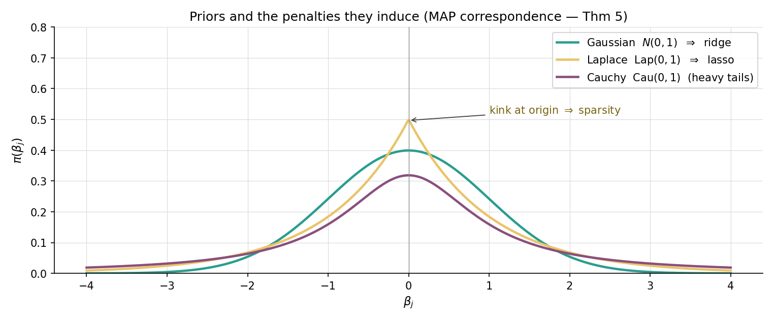
A natural extension of the Gaussian/Laplace pair is the Cauchy prior , used by Gelman et al. 2008 as a default weakly-informative prior for logistic-regression coefficients. Cauchy has heavier tails than Laplace, expressing greater prior tolerance for occasional large coefficients while still pulling small ones toward zero. The Cauchy MAP has no closed-form penalty equivalent — the resulting objective is non-convex — and requires numerical optimization. The general lesson: the Gaussian–Laplace dichotomy is the convex special case of a much richer prior-as-penalty correspondence.
Topic 14 §14.6 Rem 6 introduced Hodges superefficiency: an estimator that beats the Cramér–Rao bound at a single point (e.g. ) by being shrinkage-like there. Ridge and lasso are exactly such estimators — they have superior MSE near at the cost of bias elsewhere. Le Cam’s discrediting of superefficient estimators in the 1950s was based on their pathological behavior at non-shrinkage targets; the modern MSE-improvement view (Thm 1) reframes the same algebra as a virtue. The Stein-shrinkage origin paper (STE1956) was the first to take the bias-for-variance trade seriously; ridge and lasso are its modern descendants.
Thm 5 makes a crisp identification: is the prior precision (inverse variance) per coefficient. The empirical-Bayes view says: choose to maximize the marginal likelihood , treating as a hyperparameter of the prior. Cross-validation (§23.8) is a frequentist alternative that estimates predictive risk directly. Both procedures pick a that adapts to the data; they typically agree to within an order of magnitude, with empirical-Bayes preferring slightly smaller (less shrinkage).
In neural-network training, the term weight decay denotes the addition of to the loss — Gaussian prior MAP, by Thm 5. Equivalently, gradient-descent updates with multiplicative decay implement L² regularization for vanilla SGD (the implementation differs subtly for Adam-family optimizers, motivating decoupled weight decay in AdamW). Every modern deep-learning optimizer ships with a weight-decay knob; tuning it is one of the most reliable ways to improve generalization. Forward-pointer to formalml’s weight-decay topic.
23.8 Cross-validation for selection
The penalty parameter controls the bias-variance tradeoff. Choosing it well requires an estimate of out-of-sample predictive performance — exactly what cross-validation provides.
Partition the data into disjoint folds via a fold-assignment map . Let denote the penalized estimator trained on all data except fold . The -fold CV estimator is
where is the per-observation loss (squared error for regression, deviance for GLMs).
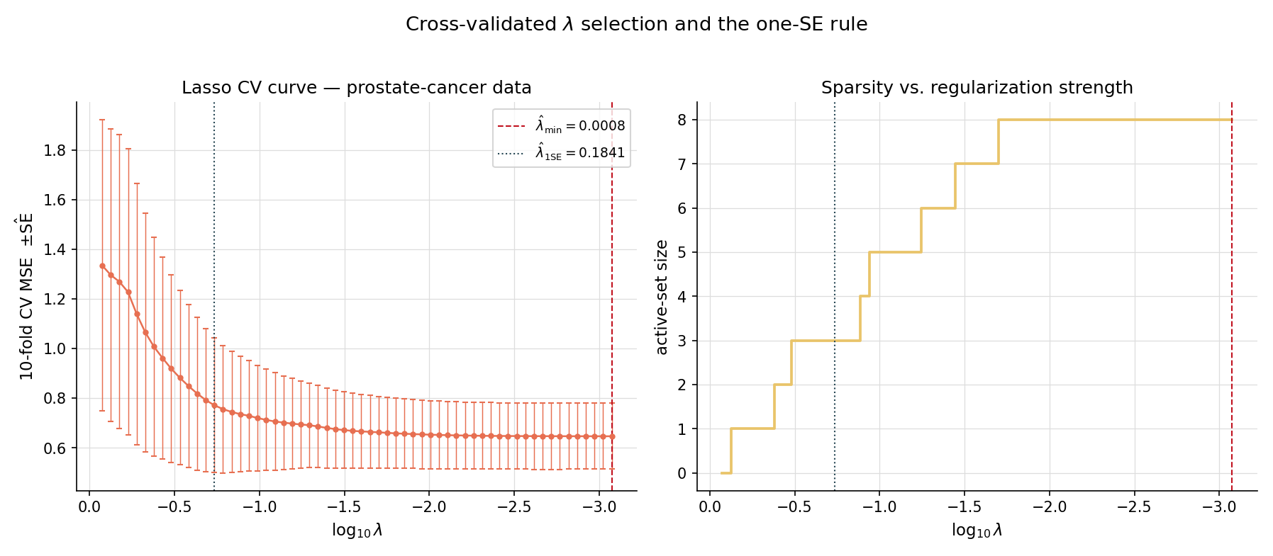
The CV curve traces a U-shape as a function of : high over-shrinks (high bias), low under-regularizes (high variance), and the minimum sits in the middle. Two standard rules pick from the curve:
- — the minimizing . Usually chosen for prediction-focused workflows.
- — the largest such that . Chooses a parsimonious model that is statistically indistinguishable from the best.
Running 5-fold and 10-fold CV on the prostate-cancer lasso path with seed 42 gives slightly different values, but typically the same order of magnitude. 10-fold CV has lower bias (more data per fit) but higher variance (smaller test folds); 5-fold has the opposite tradeoff. For , the variance of across CV runs is usually larger than the bias from choosing one over the other. 10-fold is the modern default.
On the prostate dataset, 10-fold lasso CV identifies at a small value where most of the 8 predictors enter the active set. Applying the one-SE rule shifts to a substantially larger where only 4–5 predictors remain — a sparser, more interpretable model whose CV performance is statistically indistinguishable. The one-SE rule’s aggressive bias toward sparsity is a feature when interpretation matters (e.g. variable importance for medical research) and a bug when prediction is the only goal.
cv.pathAtLambdaMin and cv.pathAtLambdaOneSE in the result struct.Letting be the empirical standard error of the per-fold deviances at , the one-SE rule is
This is Breiman, Friedman, Olshen & Stone (CART 1984) Section 3.4. The rule is deliberately conservative — it picks the sparsest model whose predictive performance falls within sampling noise of the best.
A subtle pitfall: if you choose by CV and then report the same CV curve’s minimum value as your “test error,” you’ve leaked tuning information into the test estimate. Nested cross-validation fixes this: an outer CV loop estimates generalization error, and within each outer fold, an inner CV loop selects . The outer CV’s mean error is then an honest estimate of generalization performance. Topic 24 §24.5 Rem 11 develops nested CV in the broader model-selection context; it’s mentioned here so the reader avoids the over-optimistic shortcut.
Cross-validation is one way to pick . Information criteria — AIC (), BIC (), Mallow’s — are alternatives that estimate out-of-sample risk via a complexity penalty rather than data-splitting. For penalized estimators, the effective number of parameters is replaced by the trace of the smoother matrix (ridge) or the size of the active set (lasso, with caveats). Topic 24 develops the asymptotic theory; for now the take-away is that AIC/BIC/CV typically give similar answers in the high-signal regime and diverge in the low-signal regime, with BIC favoring sparser models.
23.9 Worked examples: prostate-cancer and credit-default
This section closes the loop on the running examples by walking through two complete penalized-regression workflows.
The HTF Table 3.3 prostate-cancer dataset has 97 patients and 8 predictors; the response is lpsa. The standard workflow:
- Standardize predictors (centered and scaled to unit variance).
- Compute the regularization path on a 100-point log-grid .
- Run 10-fold CV with seed 42 to identify and .
- Refit on the full data at each chosen to get the final coefficient estimates.
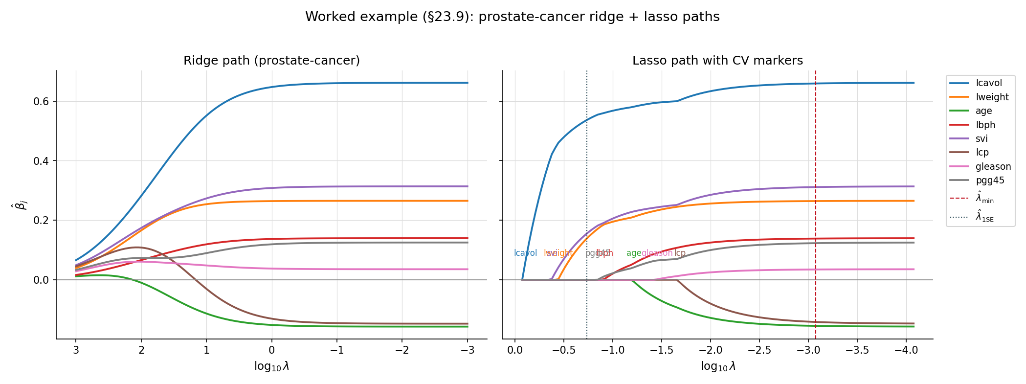
The ridge path shows smooth shrinkage: every coefficient starts near OLS at small and decays smoothly toward zero. The lasso path is piecewise linear: each coefficient enters the active set at its own , with the strongest signals (lcavol, lweight) entering first and weaker ones (gleason, pgg45) entering only at small . At , the lasso retains 4–5 predictors; ridge keeps all 8 with shrunken weights. The two estimators agree on the leading coefficients but diverge in their treatment of the marginal predictors.
Topic 22’s EXAMPLE_6_GLM_DATA has 200 observations and 2 raw predictors. Expanding to degree-3 polynomial features gives 34 columns — a high-dimensional regime where unpenalized logistic regression would overfit. Lasso-logistic regression at the CV-optimal selects 6–10 features automatically: the linear and squared terms in the original predictors, a handful of cross-terms, and a few cubic terms. The remaining polynomial features are zeroed out. This is the practical workflow that justifies the brief’s “high-dimensional p ≫ n” promise from Topic 22 §22.10 Rem 28: penalized GLMs make polynomial-feature expansion a viable modeling strategy.
A standard error: reading as if it were an unbiased estimate of . It is not. The ridge estimator is biased toward zero by design — that is the source of its variance reduction. The right interpretation: is a posterior mode under a Gaussian prior with mean zero, telling you the predictor’s contribution after regularizing for likely small effects. Lasso is even more aggressive: does not mean the predictor has no effect, just that the data doesn’t provide enough evidence to overcome the L¹ penalty’s threshold. Selected variables can be reported as “the lasso identified these as relevant,” but their numerical coefficient values should be interpreted with the bias caveat.
The penalized-estimation universe has a small number of canonical implementations:
glmnet(R, also Python viaglmnet-python) — Friedman, Hastie & Tibshirani’s reference implementation. Cyclic coord descent + warm-start path + screening rules + auto CV. The benchmark.sklearn.linear_model.{Ridge, Lasso, ElasticNet, RidgeCV, LassoCV, ElasticNetCV}(Python) — coord-descent (lasso/elasticnet) and direct solver (ridge); CV variants automate selection. Slightly slower thanglmnetfor very large but vastly more convenient for sklearn pipelines.MLJLinearModels.jl(Julia) — fast, supports a wider variety of penalties.regression.ts(this codebase) — a faithful reimplementation of the core algorithms for browser-side computation in interactive components. Not a production solver — for real workloads, use one of the above.
23.10 Forward Map
Topic 23 establishes penalized estimation as a unifying framework for stabilizing OLS and IRLS, with three penalty families (ridge, lasso, elastic net), one core algorithm (cyclic coord descent), and one selection procedure (cross-validation). The forward map below catalogs where the framework leads.
Let have at most nonzero components and assume satisfies the restricted eigenvalue condition with constant . Then for , the lasso estimator satisfies
The rate is information-theoretically optimal up to constants — the lasso is minimax-rate optimal under sparsity. WAI2019 Thm 7.13 (statement adapted). Not proved here; the full development (RIP, RE conditions, dual certificates) is at formalml.
The next Track 6 topic generalizes selection to a broader model selection framework. AIC () estimates expected out-of-sample log-likelihood; BIC () approximates the Bayesian marginal likelihood; Mallow’s is the Gaussian special case of AIC. Stone 1977 identifies LOO-CV with AIC asymptotically; Yang 2005 proves selection consistency and prediction efficiency are formally incompatible. Topic 24 develops the asymptotic theory and the trade-offs.
Thm 5’s MAP-as-penalized-MLE correspondence is the gateway to the Bayesian treatment of regularization. Topic 25 §25.7–§25.8 develops prior selection (Jeffreys, weakly-informative, improper with integrable posterior) and shows MAP-as-penalized-MLE as Ex 8. Topic 28 (Hierarchical Bayes) develops hierarchical priors that learn from the data (empirical-Bayes ridge) and modern continuous shrinkage priors like the horseshoe (Carvalho–Polson–Scott 2010), which approximate lasso’s sparsity behavior with a globally adaptive scale. The horseshoe is, in a sense, the “lasso of priors.”
Several practical generalizations of lasso are catalogued in HTW2015:
- Group lasso (Yuan & Lin 2006): penalty for predefined predictor groups, performing group-level selection.
- Fused lasso (Tibshirani et al. 2005): penalty for ordered coefficients, encouraging piecewise-constant fits — used in genomics and signal denoising.
- Sparse-group lasso (Simon et al. 2013): combines L¹ within groups and L² across groups.
These are non-separable penalties (the fused-lasso term couples adjacent coefficients), so cyclic CD doesn’t apply directly — proximal-gradient or ADMM is the standard solver. Track 8 covers the algorithms and theory.
Lasso has known biases at large coefficients — its constant L¹ shrinkage applies even when the data overwhelmingly support a strong nonzero effect. SCAD (Smoothly Clipped Absolute Deviation; Fan & Li 2001) and MCP (Minimax Concave Penalty; Zhang 2010) are non-convex penalties designed to give lasso-like sparsity for small coefficients but no shrinkage for large ones. The trade-off is computational: the resulting objective is non-convex, requiring local-linear-approximation algorithms or proximal-gradient methods with careful initialization. SCAD/MCP estimators have the oracle property — they perform as if the true active set were known a priori — under regularity conditions. The methodology is mature; Topic 23 leaves it as a deferral pointer (FAN2001).
The asymptotic theory of penalized estimation in regimes is the domain of high-dimensional statistics. The key tools are oracle inequalities (Bickel–Ritov–Tsybakov 2009), restricted-eigenvalue conditions (Bickel et al. 2009), and the dual-certificate technique. The debiased lasso (Javanmard–Montanari 2014; van de Geer et al. 2014) gives valid post-selection confidence intervals by adding a one-step Newton correction to the lasso estimate. Double descent (Belkin et al. 2019) shows that predictive risk can have a second descent past the interpolation threshold — overparameterization is not always overfitting. All of this lives at formalml’s high-dimensional regression topic.
Modern deep learning training relies heavily on weight decay — Thm 5’s Gaussian-prior MAP applied to neural-network weights. The SGD-with-decay update implements L² regularization; the more-complicated AdamW decoupling separates weight decay from the adaptive learning rate. Implicit regularization — the bias of SGD toward minimum-norm solutions in overparameterized regimes — plays the role of explicit ridge in modern practice, often with no tuning required. The connection to Topic 23 is direct: every deep-learning regularizer is a penalty, every penalty is a prior, and the bias-variance tradeoff still rules.

Topic 23 closes Track 6’s main framework. Linear regression (Topic 21) is OLS as orthogonal projection. GLMs (Topic 22) are IRLS on the exponential family. Penalized estimation (this topic) is what you reach for when those frameworks break — collinearity, separation, . Topic 24 closes Track 6 with the model-selection layer that picks which features to include in the first place; reciprocally, the -indexed family of this topic IS a continuous model space with effective DOF — Topic 23 is a special case of Topic 24’s framework. Together, Topics 21–24 cover the full classical-regression toolkit; Tracks 7–8 and formalml.com take it from there.
References
- Hoerl, A. E. & Kennard, R. W. (1970). Ridge regression: Biased estimation for nonorthogonal problems. Technometrics, 12(1), 55–67.
- Tikhonov, A. N. (1943). On the stability of inverse problems. Doklady Akademii Nauk SSSR, 39(5), 195–198.
- Tibshirani, R. (1996). Regression shrinkage and selection via the lasso. Journal of the Royal Statistical Society, Series B, 58(1), 267–288.
- Zou, H. & Hastie, T. (2005). Regularization and variable selection via the elastic net. Journal of the Royal Statistical Society, Series B, 67(2), 301–320.
- Friedman, J., Hastie, T. & Tibshirani, R. (2010). Regularization paths for generalized linear models via coordinate descent. Journal of Statistical Software, 33(1), 1–22.
- Tseng, P. (2001). Convergence of a block coordinate descent method for nondifferentiable minimization. Journal of Optimization Theory and Applications, 109(3), 475–494.
- Hastie, T., Tibshirani, R. & Friedman, J. (2009). The Elements of Statistical Learning (2nd ed.). Springer.
- Hastie, T., Tibshirani, R. & Wainwright, M. (2015). Statistical Learning with Sparsity: The Lasso and Generalizations. Chapman & Hall/CRC.
- Stein, C. (1956). Inadmissibility of the usual estimator for the mean of a multivariate normal distribution. Proceedings of the Third Berkeley Symposium on Mathematical Statistics and Probability, Vol. 1, 197–206. University of California Press.
- Firth, D. (1993). Bias reduction of maximum likelihood estimates. Biometrika, 80(1), 27–38.
- Fan, J. & Li, R. (2001). Variable selection via nonconcave penalized likelihood and its oracle properties. Journal of the American Statistical Association, 96(456), 1348–1360.
- Wainwright, M. J. (2019). High-Dimensional Statistics: A Non-Asymptotic Viewpoint. Cambridge University Press.
- Lehmann, E. L. & Romano, J. P. (2005). Testing Statistical Hypotheses (3rd ed.). Springer.
- Casella, G. & Berger, R. L. (2002). Statistical Inference (2nd ed.). Duxbury.