Point Estimation & Bias-Variance
Estimators as random variables, bias, variance, MSE decomposition — the framework for evaluating any estimator.
13.1 Estimators as Random Variables
Every inferential procedure you have ever run — a sample mean, a regression coefficient, a p-value, a posterior mode — was computed from data. Before the data arrived, that computation was a function waiting for input. After the data arrives, it returns a number. That number feels concrete, but the procedure that produced it is the object of interest, and the procedure is a random variable: its value depends on which sample happened to land in your hands. Different samples, different value. An estimator is not a single number; it is a distribution, summarized in the long run by a single number plus some scatter.
This shift in viewpoint is the entire foundation of estimation theory. We stop asking “what number did I compute?” and start asking “what distribution does my computation have, and what does that distribution say about the parameter I care about?” The distribution of an estimator across repeated sampling is called its sampling distribution. Bias, variance, MSE, consistency, efficiency — every concept in this topic is a property of that sampling distribution.
A statistic is any measurable function of the observed sample. Equivalently, is a random variable whose value is determined by the data, and whose distribution is induced by the joint distribution of the sample.
“Measurable” is a technical requirement — it ensures probabilities of events like are well-defined — and is satisfied by every computation a human could plausibly write down. The key restriction is that must depend only on the data, not on unknown parameters. So is a statistic; so is or . But is not a statistic when is the unknown parameter we are estimating: it involves the quantity we are trying to learn.
A point estimator of a parameter is a statistic whose value is used as a guess for . The estimator is a random variable; its value for a particular sample realization is a point estimate.
The distinction between estimator and estimate is the same as that between the function and its value. “The sample mean” is an estimator — a recipe applicable to any sample. “The sample mean of our data, which equals ” is an estimate — the recipe evaluated on a specific sample. Almost every confusion in introductory statistics traces back to conflating these. When we ask “is this estimator unbiased?” we are asking about the recipe across all possible samples, not about any particular number.
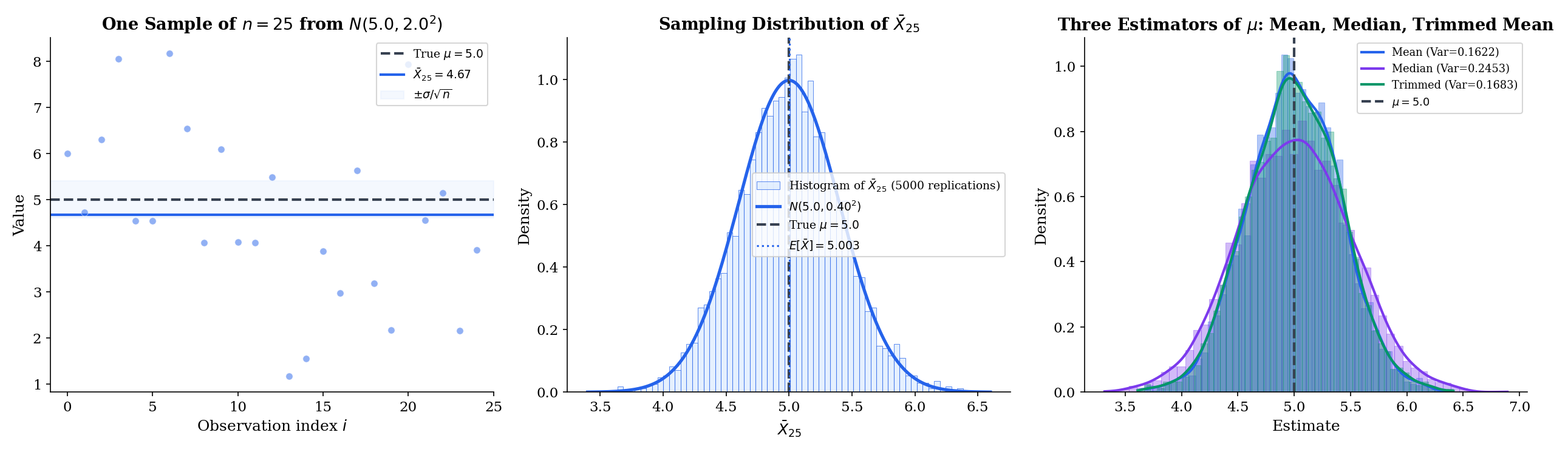
Suppose are iid with unknown mean and finite variance. Three candidate estimators of :
- Sample mean: .
- Sample median: , the middle order statistic — whose asymptotics are developed in Topic 29 §29.6.
- Trimmed mean: = mean of the sample after discarding the top and bottom of observations.
All three are statistics (they depend only on the data), all three target the same , and all three are reasonable candidates. They produce different values on the same sample, and their sampling distributions are different shapes. Which one is “best” depends on the underlying distribution and on what we mean by “best” — the rest of this topic builds the vocabulary to answer that question precisely.
In an introductory statistics class, you compute the sample mean of a dataset and report it as “the” estimate. In estimation theory, we take one step back and ask: if we could repeatedly draw fresh samples of size from the population and compute the sample mean each time, what distribution of values would we see? That distribution — not any single computed value — is the object we analyze. Its center is where our estimates cluster on average (bias tells us whether that center is ). Its spread tells us how precise any single estimate is (variance). Its shape tells us how the estimator behaves in the tails, and for large , what confidence intervals look like (asymptotic normality). Every theorem in this topic is a statement about that distribution.
This is also why we write with a hat: the hat signals “random variable, function of the data,” distinguishing it from the unknown-but-fixed true parameter . Reading a formula, always ask: which symbols are random? which are fixed? The answer changes everything.
| MC | Theory | |
|---|---|---|
| E[θ̂] | — | 5.0000 |
| Bias | — | 0.0000 |
| Variance | — | 0.1600 |
| MSE | — | 0.1600 |
| SE | — | 0.4000 |
13.2 Bias
The first criterion for a “good” estimator is simple: on average, across repeated sampling, does it hit the target? An estimator whose expected value equals the true parameter is called unbiased. Unbiasedness sounds like a bedrock virtue, but as we will see in §13.4, it is surprisingly easy to do better by being deliberately biased. First, the definitions.
Let be an estimator of . Its bias is the difference between its expected value and the true parameter:
The expectation is taken over the sampling distribution of , treating as fixed.
Bias measures a systematic error: if bias is positive, the estimator overestimates on average; if negative, it underestimates. Random error — the deviation of any particular estimate from — is captured by variance, which §13.3 develops.
The estimator is unbiased for if , equivalently , for every value of in the parameter space.
![Three-panel bias visualization: (left) a dart-board analogy contrasting high-bias/low-variance, low-bias/high-variance, and low-bias/low-variance clusters; (center) Bessel's correction — E[S²] with 1/n (biased) vs 1/(n−1) (unbiased) as n grows; (right) MSE comparison of the two sample-variance estimators](/images/topics/point-estimation/bias-visualization.png)
The universal quantifier — for every value of — matters. A procedure that happens to return the right answer for but systematically misses for other values is not unbiased in this technical sense. Unbiasedness is a property of the estimator’s behavior uniformly across the parameter space, not at any single point.
If are iid with (assumed finite), then the sample mean is unbiased for :
Proof [show]
Start from the definition of the sample mean:
By linearity of expectation — which does not require independence — we can pull the constant outside and distribute the expectation across the sum:
Because the are iid, each , and there are copies:
The proof is two lines, but the two ingredients — linearity of expectation and identical means — are the template for essentially every unbiasedness calculation you will ever do.
The iid assumption in Theorem 1 is stronger than needed: we only used that for every . So the sample mean is unbiased whenever the summands share a common mean, even if their variances differ or their distributions are different. For example, if and both have mean , then is still unbiased for . Unbiasedness of linear statistics is astonishingly robust.
Contrast this with the sample median, which is not generally unbiased for unless the distribution is symmetric around . For Exponential, the population mean is but the population median is ; the sample median is unbiased for the median, not the mean.
The natural candidate for estimating the population variance is the average squared deviation from the sample mean:
This is the maximum-likelihood estimate of when the underlying distribution is Normal, and it is the “natural” variance of the empirical distribution. But it is biased. A direct calculation — expanding the squared deviation, using (Theorem 2 below), and collecting terms — shows
So underestimates by a factor of . The fix is to divide by instead of :
This is the unbiased sample variance, and the denominator is called Bessel’s correction. The correction is intuitive: in computing from the data we have “used up” one degree of freedom, so only independent residuals remain. The unbiasedness of follows immediately: .
Which divisor should you use in practice? That turns out to be a more subtle question than it first appears — see Example 5 in §13.4.
Unbiasedness feels like a bedrock virtue, but consider the estimator — the first observation, ignoring everything else. It is unbiased for : . It is also a terrible estimator: its variance is , compared with for the sample mean, so after any real amount of data it is times worse. Unbiasedness is satisfied; precision is not.
More dramatically, some parameters admit no unbiased estimator at all (e.g., the reciprocal of a Poisson mean), while others admit only pathological ones. And, as we will see, biased estimators can systematically outperform unbiased ones in mean squared error — shrinkage estimators, ridge regression, and James–Stein all exploit this. Unbiasedness is one input into evaluation, not the whole story. The right criterion combines bias and variance, which is what MSE does.
13.3 Variance and Standard Error
The second criterion for a “good” estimator is precision: how spread out is the sampling distribution? If two estimators are both unbiased but one has half the variance, it gives estimates that are closer to the truth on average — by a lot. The standard measure of spread for an estimator is its standard deviation, which in this context has a special name.
The standard error of an estimator is the standard deviation of its sampling distribution:
When the estimator’s variance depends on unknown population parameters, the estimated standard error plugs in sample-based substitutes.
The word “standard error” exists because we needed a term distinct from “standard deviation of the population.” Standard deviation describes the spread of the underlying random variable . Standard error describes the spread of an estimator computed from many ‘s — which is almost always much smaller, thanks to averaging.
If are iid with (assumed finite), then the sample mean has variance
and therefore standard error .
Proof [show]
Expand the sample mean as a scaled sum:
By independence, variance distributes over a sum:
Substituting:
The factor of is the entire content of the sample mean’s appeal. It says that doubling the sample size halves the variance — precision improves linearly in . And the factor of in the standard error is the rate at which confidence intervals narrow, the rate that appears in the CLT, and the rate that organizes almost all of classical statistics.
If are iid , the sample mean satisfies exactly — no approximation, no CLT needed. Its standard error is . For and , that is : a single sample mean will typically land within of (about one SE), and almost always within (two SEs).
When is unknown — the usual case — we plug in the sample standard deviation (from Example 3) to get the estimated standard error . The distinction matters: confidence intervals built from use the Student’s distribution, not the standard Normal, because introduces additional uncertainty. That -correction is Topic 11’s Example 7, and the machinery of confidence intervals will develop it systematically.
It is easy to conflate “standard deviation” and “standard error.” The difference is crucial:
- The standard deviation describes the spread of the population. It does not shrink as you collect more data.
- The standard error describes the spread of the estimator. It shrinks like .
When you report a sample mean as ”,” the is the standard error — how uncertain you are about the mean. When you report that your data has standard deviation , that is the standard deviation — how spread out the individual observations are. SE says how precisely you know the average; SD says how dispersed the raw data are. SE is precision about precision — a derived uncertainty.
13.4 Mean Squared Error and the Bias-Variance Decomposition
Bias and variance are both measures of estimator quality, and they are in tension: biased estimators can have lower variance, and vice versa. We need a single scalar that combines both. The natural choice — and the one whose properties organize the entire remainder of this topic — is the mean squared error.
The mean squared error of an estimator of is the expected squared deviation from the truth:
The expectation is taken over the sampling distribution of , treating as fixed.
MSE is the squared analog of bias — instead of asking “how far off is the estimator on average?” it asks “how far off squared is the estimator on average?” Squaring turns the signed error into a positive quantity and penalizes large deviations more severely, which makes MSE a natural loss function. Crucially, MSE decomposes into a systematic part (bias squared) and a random part (variance), making the tradeoff between the two explicit.
For any estimator of with finite second moment,
Equivalently, splits cleanly into a mean-offset term and a dispersion term.
Proof [show]
The trick is to add and subtract the mean inside :
The first parenthesis is the random deviation of from its mean — its variance comes from here. The second parenthesis is the systematic deviation of the mean from the truth — the bias. Square both sides:
Now take expectations. The first term becomes by definition:
The middle term vanishes. To see this, pull out , which is a constant with respect to the expectation, leaving :
The third term is already deterministic — it is the square of the bias:
Collecting:
The proof is the same “add and subtract the mean” maneuver that powered the variance decomposition in Topic 4 (Eve’s law), and it gives the central identity of estimation theory. An unbiased estimator pays all of its MSE as variance. A highly precise but biased estimator pays most of its MSE as bias squared. Minimizing MSE means navigating the tradeoff between the two — which is what the rest of this topic is about.
![Three-panel bias-variance tradeoff for polynomial regression: degree 1 (underfitting, high bias), degree 5 (good fit), degree 15 (overfitting, high variance). Each panel shows 50 training-set fits overlaid, the average fit E[f̂(x)] in bold, and the Bias²/Var/MSE values](/images/topics/point-estimation/bias-variance-tradeoff.png)
From Example 3, the two candidates for estimating are:
- , unbiased.
- , biased with .
For iid Normal data, it can be shown that and . Plugging into the MSE decomposition:
For : vs. . The biased estimator has lower MSE. This is not a trick: Bessel’s correction removes bias at the cost of increased variance, and the tradeoff does not always favor unbiasedness. It turns out that — shrinking even more aggressively than the MLE — has smaller MSE still for Normal data. Minimum-MSE and unbiasedness are genuinely different objectives.
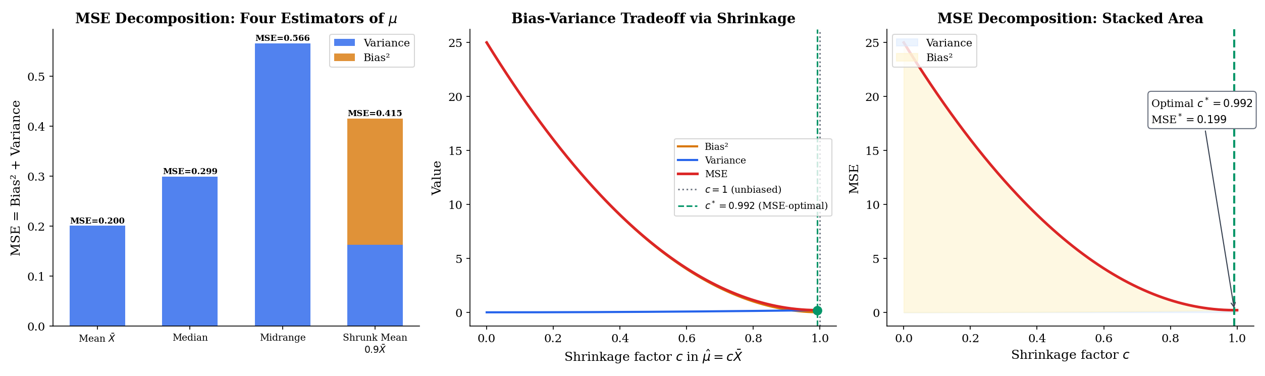
Consider estimating from iid data with the family of shrinkage estimators
At we recover the sample mean (unbiased, MSE ). At we get the trivial estimator that always returns zero (biased by , variance zero, MSE ). In between, bias and variance trade off:
Differentiating with respect to and setting to zero gives the MSE-optimal shrinkage
Note that strictly whenever — which it always is. So the sample mean is never MSE-optimal in this family; there always exists a shrunk version that strictly dominates it. The catch: depends on itself, so we cannot use it as a standalone estimator. But this example is the seed of every shrinkage, regularization, and empirical-Bayes method: allowing bias opens a strictly better option in terms of MSE.
Theorem 3 makes the bias-variance tradeoff precise: MSE has two components, and reducing one often increases the other. This is not a metaphor — it is an algebraic identity. Every strategy for minimizing MSE must navigate this tension:
- More data (): variance shrinks like , bias typically unaffected. So MSE is dominated by bias at large — unbiased consistent estimators eventually win.
- Simpler models / more shrinkage: bias increases, variance decreases. Good for small when variance dominates.
- More flexible models / less shrinkage: bias decreases, variance increases. Good for large when bias dominates.
In an ML context, this is the polynomial-fitting story: a degree-1 line is highly biased but low-variance; a degree-15 polynomial is nearly unbiased but enormously variable. Regularization, cross-validation, and model selection all exist to find the sweet spot. Section 13.9 develops the ML connection in detail.
13.5 Consistency
The properties so far — bias, variance, MSE — are finite-sample statements: they hold for every . The next two sections zoom out and ask: what happens as ? Does the estimator settle down to the truth? Does its sampling distribution take a recognizable shape? Consistency answers the first question, and we already have all the machinery we need — the law of large numbers does almost all of the work.
An estimator is consistent for if, as , it converges to in probability: for every ,
Equivalently, .
Consistency is the minimal requirement for an estimator to be useful at large sample sizes. If is inconsistent, then even infinite data will not push it to the right answer; no amount of precision can compensate for a procedure that is aimed at the wrong target asymptotically. Unbiasedness and consistency are logically independent (Remark 5), so we need both words.
An estimator is strongly consistent for if : the set of sample sequences on which the running estimates fail to converge to has probability zero.
Strong consistency implies consistency (convergence almost sure implies convergence in probability, per Topic 9), so whenever the strong law of large numbers applies we get strong consistency “for free.” The distinction matters most when we track a single infinite sequence of data, as a streaming algorithm would — strong consistency guarantees the stream’s running estimate eventually stays close to the truth, not just that any given sample-size- snapshot is likely to be close.
If as , then is consistent for .
Proof [show]
By Chebyshev’s inequality applied to the random variable , for any :
By hypothesis , so the right-hand side tends to for every fixed . Therefore
which is the definition of consistency.
Because MSE decomposes as bias² + variance, Theorem 4 gives a two-part recipe: if and , then is consistent. This is the most common way to prove consistency in practice — check that bias vanishes and variance shrinks. For the sample mean, bias is zero for all and variance is , so consistency is immediate — but the theorem gives us a cleaner route via the LLN.
If are iid with and , then the sample mean is strongly consistent for :
If only is known, the weaker statement follows from Chebyshev (Theorem 4 above) or from the weak law of large numbers.
This is the strong law of large numbers from Topic 10, restated in estimator language. The sample mean is the prototypical consistent estimator, and the LLN is the engine: consistency of the sample mean is literally the LLN under a different name. Every estimator that can be written as (or derived from) a sample mean inherits consistency from the LLN — this is the template that Maximum Likelihood Estimation uses to prove the MLE is consistent, and Topic 15 uses to handle method-of-moments estimators.
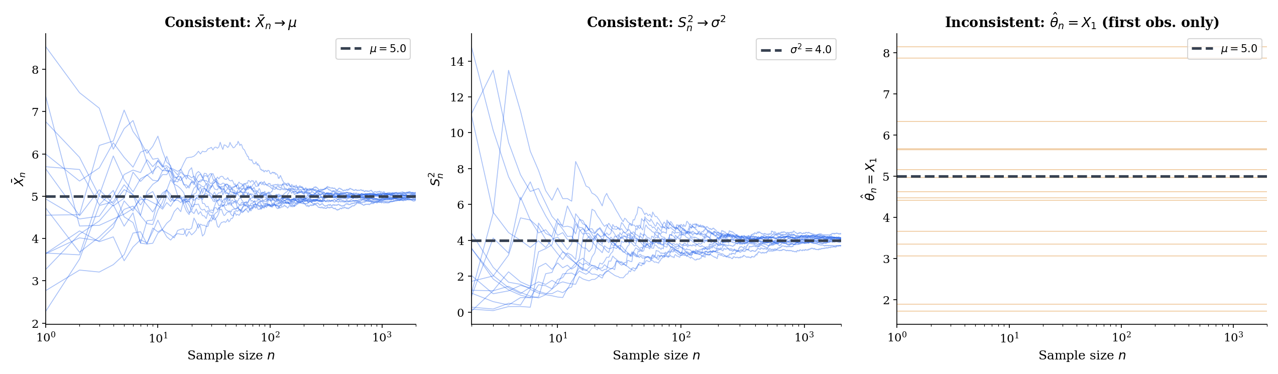
Let be iid with (a fourth-moment condition, stronger than what Theorem 5 required). The unbiased sample variance is consistent for .
Sketch. Expand
By the LLN applied to , the first average converges almost surely to . By the LLN applied to and continuous-mapping, . The factor . Combining:
Consistency of the biased version follows immediately by the same argument (multiplying by ). Both divisors yield consistent estimators of ; they differ only in finite-sample MSE.
Consider the estimator of the population mean . It is unbiased (), but it ignores all but the first observation — no matter how many data points you collect, the estimate never updates after .
Formally: does not depend on at all, so — a fixed, positive number for any and any non-degenerate distribution. The probability does not shrink with . Therefore is inconsistent, despite being unbiased.
This is the cleanest demonstration that unbiasedness and consistency are independent properties. has for every , which does not shrink, so Theorem 4 does not kick in.
Examples 7 and 8 make the point: consistency and unbiasedness are logically independent. Exhaustive possibilities:
- Both: sample mean, unbiased sample variance. The ideal case.
- Unbiased, inconsistent: . Unbiased but fails to improve with more data.
- Biased, consistent: biased sample variance . Its bias shrinks as (), so it is asymptotically unbiased; with vanishing variance, it is consistent.
- Neither: the constant estimator (or any fixed value unrelated to ). Ignores the data, biased except by coincidence, not consistent.
For practical purposes, consistency is the more important of the two: we typically want an estimator that eventually gets the right answer, and we tolerate small-sample bias as long as it washes out. Unbiasedness is sometimes useful as a finite-sample property (e.g. for building exact confidence intervals under Normal assumptions), but asymptotic unbiasedness — — is what modern statistics actually requires most of the time.
13.6 Asymptotic Normality
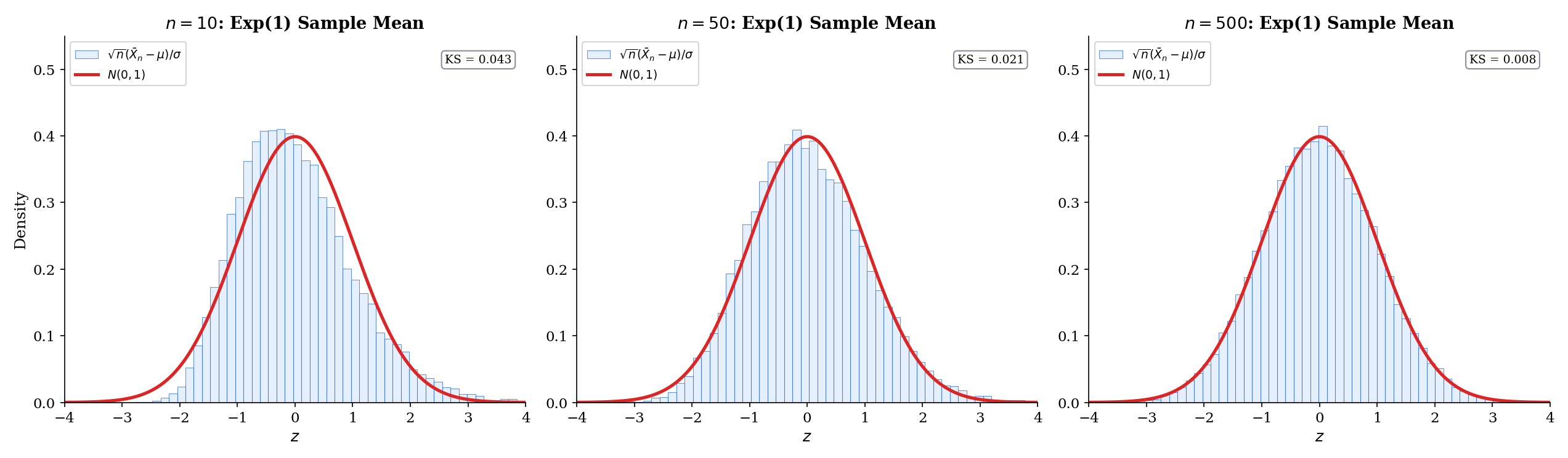
Consistency tells us eventually lands near . Asymptotic normality tells us what its shape is near : for large , the sampling distribution is approximately Gaussian, with a known variance. This is what powers confidence intervals, z-tests, and t-tests. The central limit theorem is the engine here, and — as with consistency and the LLN — most of the work is already done.
The estimator is asymptotically normal with asymptotic variance if
where denotes convergence in distribution. Informally, for large , .
The factor is essential. Without it, (by consistency) and the limit distribution would be a point mass at zero — degenerate and useless. The scales the fluctuations up at the right rate so the limit is non-degenerate. The asymptotic variance is the “per-sample” variance at the scale — what the histogram of converges to.
If are iid with , then the sample mean is asymptotically normal with asymptotic variance :
This is the classical CLT of Topic 11, restated as an estimator result. The only change is language: instead of “sums and averages converge to a Gaussian,” we say “the sample mean is an asymptotically normal estimator of with asymptotic variance .” The quantities are identical; the framing is new.
Let be asymptotically normal: . Let be differentiable at with . Then is asymptotically normal for :
The delta method is the workhorse for deriving asymptotic distributions of non-linear functions of estimators. It says that smooth transformations inherit asymptotic normality, with variance rescaled by the squared derivative of the transformation — a first-order Taylor expansion at the asymptotic regime. The proof is in Topic 11 (Theorem 11.8); we will apply it repeatedly in Topics 14 and 15 to handle things like (when estimating a rate) and (when estimating a squared quantity).
We want the limit distribution of for iid data with finite fourth moment. Write the sample variance as a function of two sample means: where .
By the multivariate CLT applied to the random vector , the vector is jointly asymptotically Normal around with a covariance matrix determined by the first four moments of . Applying the delta method to :
where is the central fourth moment. For Normal data, , so the asymptotic variance simplifies to — which matches the exact (small-sample) variance formula from Example 5 after the rescaling. For non-Normal data, the formula picks up the excess kurtosis: heavier tails mean the sample variance has larger asymptotic variance, because extreme observations dominate the squared residuals.
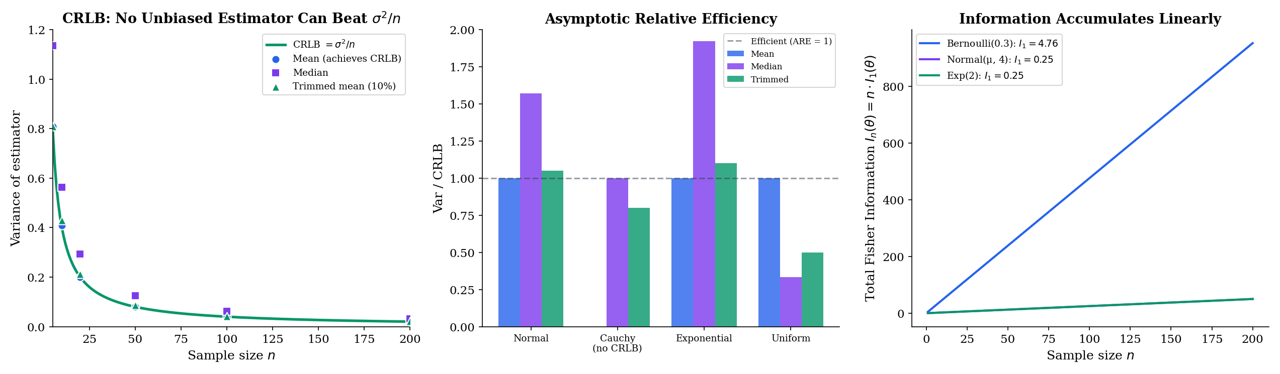
Asymptotic normality gives us an apples-to-apples way to compare estimators: look at their asymptotic variances. For two asymptotically normal estimators and of the same parameter, the asymptotic relative efficiency is
the ratio of their asymptotic variances (in the order that makes values above mean ” wins”). For Normal data, the sample median has ARE relative to the sample mean — meaning 1,000 observations for the median give about the same precision as for the mean. For Cauchy data (where the sample mean has no well-defined asymptotic variance), the ARE comparison flips: the median is the efficient choice and the mean is catastrophic. Asymptotic efficiency is distribution-dependent; efficient-for-Normal and efficient-for-Cauchy are different estimators.
The next section, on the Cramér–Rao bound, quantifies the ceiling on achievable asymptotic variance — and therefore the ceiling on asymptotic efficiency.
13.7 Efficiency and the Cramér-Rao Lower Bound
We have seen that bias and variance trade off, and that asymptotic variance gives us a clean way to compare estimators. The natural next question: how small can the variance of an unbiased estimator possibly be? Is there a fundamental floor, or can clever procedures improve without limit? The answer is the Cramér–Rao lower bound — the most important non-trivial inequality in estimation theory. It says that the variance of any unbiased estimator is bounded below by a quantity depending only on the model (the distribution family) and the parameter — the Fisher information.
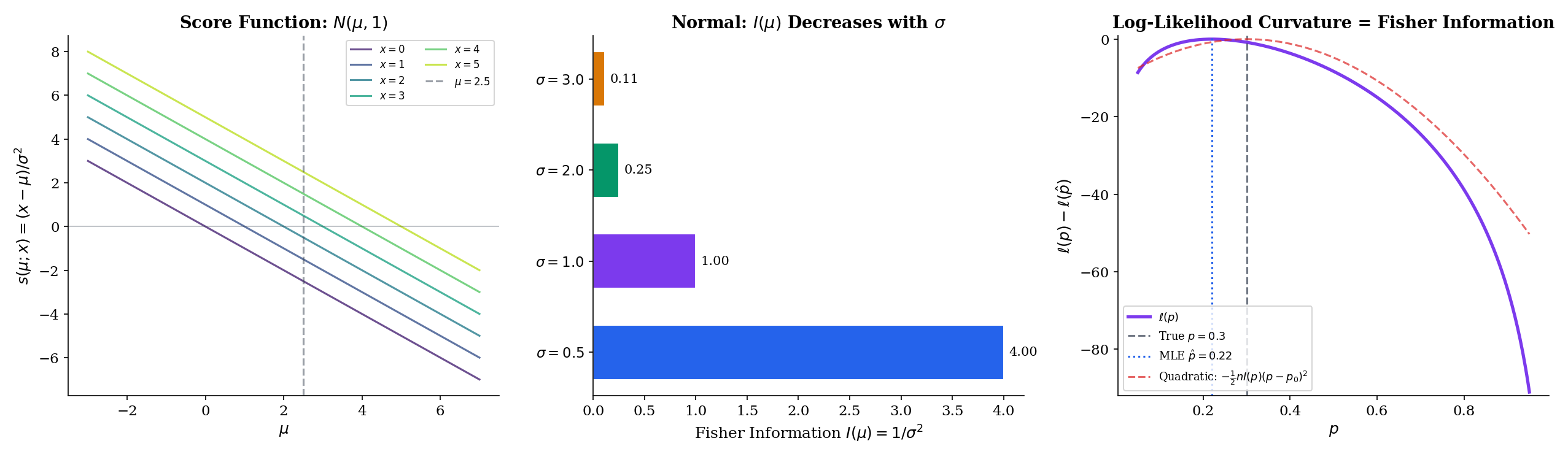
Let be a parametric family of densities (or PMFs) with . The score function is the partial derivative of the log-likelihood with respect to the parameter:
For an iid sample, the total score is the sum of per-observation scores: .
The score is the “sensitivity of the log-likelihood to the parameter, at a given data point.” It is a random variable (depends on ); for a well-specified model, its expected value at the true parameter is zero. The maximum-likelihood estimator is defined as the that makes the total score zero. Score-based methods (score tests, score matching, efficient-score GLMs) pervade modern statistics.
The Fisher information at is the variance of the score:
Under regularity conditions, an equivalent form is the negative expected second derivative of the log-likelihood:
Fisher information measures how much information one observation carries about — equivalently, how curved the log-likelihood is near the true parameter. Sharp curvature (high ) means the log-likelihood is a steep parabola near its peak: small changes in produce large changes in log-likelihood, so the data is highly informative about . Flat curvature (low ) means the log-likelihood is nearly level: data poorly discriminates among candidate ‘s. Fisher information is additive for iid samples: observations carry total information.
Under regularity conditions that allow interchange of differentiation and integration,
Proof [show]
Start from the fact that is a density for every , so it integrates to :
Differentiate both sides in . The regularity conditions are exactly what justify swapping the derivative and the integral:
Rewrite :
which is the first claim. For the second, differentiate again:
Substitute into the second term:
which says
The second term is by the first claim. So
Theorem 8 gives the two definitions of — as the variance of the score, or as the negative expected curvature — and shows they are equal. This is what makes Fisher information computable in practice: for many distributions, the second derivative of the log-likelihood is easier to evaluate than the squared first derivative.
An unbiased estimator whose variance attains the Cramér–Rao lower bound (Theorem 9) for every is called efficient. An asymptotically normal estimator whose asymptotic variance attains the asymptotic Cramér–Rao bound is called asymptotically efficient.
Let be an unbiased estimator of based on an iid sample of size from a parametric family satisfying the regularity conditions. Then
Proof [show]
The proof applies the Cauchy–Schwarz inequality to the covariance of with the total score .
Step 1. Unbiasedness says for every , i.e. , where and . Differentiate in , swapping differentiation and integration by the regularity conditions:
Step 2. Because (Theorem 8 applied to each term and summed), the product equals the covariance:
Step 3. Apply the Cauchy–Schwarz inequality to the covariance:
By independence of the , . Substituting from Step 2:
Step 4. Rearranging,
The Cramér–Rao proof is a masterclass in statistical reasoning: an identity ( for unbiased estimators) plus an inner-product inequality (Cauchy–Schwarz) plus independence-additivity of variance yield the floor on estimator precision. The bound is achieved — the inequality becomes equality — when is proportional to , which happens for sample means of distributions in exponential families. This is the link between the Cramér–Rao bound, efficient estimation, and exponential families that Topic 16 will develop in full.
Three canonical computations using :
Normal with respect to (known ): . Two derivatives: . Taking the negative expectation (which is constant):
The Fisher information does not depend on , only on : narrow distributions carry more information per sample about their location.
Bernoulli: . Second derivative . Expectation: . Negating:
Fisher information is maximized at (where variance is highest and is least predictable) and diverges as or — near the boundary, each observation is enormously informative about whether is exactly or exactly .
Exponential: for . Second derivative . Negating:
Larger rate means faster decay, which means observations cluster near zero and carry more information about .
For iid with known , the sample mean is unbiased and has variance (Theorem 2). From Example 10, . The Cramér–Rao lower bound is
Equality. The sample mean is the efficient estimator of the Normal mean — no unbiased estimator based on iid Normal observations can do better. This is the canonical result that motivates the CRLB in the first place, and the reason the sample mean is the point estimator you reach for whenever Normality is plausible. For non-Normal data the sample mean is still unbiased and consistent, but it may no longer be efficient — the median beats it for Cauchy, and trimmed means dominate for heavy-tailed distributions.
The Cramér–Rao proof requires regularity conditions that allow interchange of differentiation and integration. Informally: the support of must not depend on , and must be well-behaved enough to differentiate under the integral. These conditions hold for essentially every standard family — Normal, Poisson, Bernoulli, Exponential, Gamma, Beta — but fail in a few important cases:
- Uniform: the support is , which depends on . The MLE has variance , faster than the rate the CRLB would predict. The CRLB does not apply.
- Shifted exponentials: for . Same issue — boundary of the support moves with .
- Heavy-tailed distributions with infinite Fisher information (Cauchy w.r.t. scale, for instance): the bound is , which is trivially satisfied but uninformative.
When regularity holds, the CRLB is the ceiling: no unbiased estimator can beat . When regularity fails, different tools — the theory, order-statistics asymptotics (Topic 29 §29.6), the Hájek-Le Cam framework — take over. For standard statistical modeling, regularity holds and the CRLB is the right benchmark.
13.8 Comparing Estimators: Admissibility and Minimax
So far we have compared estimators by MSE at a single value of . But is unknown, and a procedure that is great at one value and terrible at others is not a good procedure. Decision theory — the framework that organizes this comparison — asks: is uniformly at least as good as ? When no estimator is uniformly best, how do we choose among incomparable ones? This section introduces the key concepts (admissibility, minimax) and then presents the famous result — Stein’s paradox — that the “natural” estimator is sometimes provably dominated by something stranger.
An estimator is dominated by if for all , with strict inequality for at least one . An estimator that is not dominated by any other is admissible.
Admissibility is a weak criterion — it only says that no estimator is uniformly better. An admissible estimator can still be terrible (the constant estimator is admissible in every problem: no other estimator can dominate it, because is a point where “always guess 7” has zero MSE). Conversely, inadmissibility is a serious charge: if there exists a uniform improvement, any rational statistician should use it.
An estimator is minimax if it minimizes the maximum risk:
Minimax estimators are conservative: they trade off finite-sample performance at typical parameter values for worst-case robustness.
Minimax is a pessimistic criterion — minimize the damage in the worst case — and it frequently produces estimators that are not the best on average. Bayesian estimators are often preferable when some prior on is available. In most applied work, MSE at a point estimate of is the right loss and minimax is overcautious.
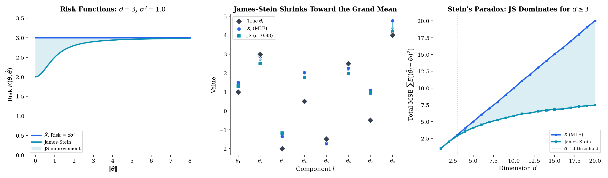
Let with unknown mean vector and known scale . For , the James–Stein estimator
has strictly smaller total MSE than the sample mean for every value of :
Therefore the sample mean is inadmissible in dimension .
Proof [show]
Proof sketch. The full proof uses Stein’s lemma — integration by parts for Normal expectations — to compute in closed form. Here we give the statement and the geometric intuition.
Statement. An explicit (slightly idealized) risk formula for the non-positive-part James–Stein estimator is
which is strictly less than (the risk of the MLE) for every , provided . The positive-part version is uniformly at least as good.
Geometric intuition. The sample mean estimates each component independently. In dimensions, the “noise ball” around concentrates in a thin annulus at radius — by the CLT applied to . Shrinking toward the origin (or any fixed point) reduces total squared error on average, because the shrinkage moves most of the noise away from the part of the annulus farthest from the origin, more than it moves signal away from the target. The factor is the smallest shrinkage strength that wins against noise in all directions simultaneously — it is exactly the threshold where the bound integrates to give a net improvement.
Pointer. The full proof uses Stein’s identity: for and smooth , . Applied coordinate-wise to the squared error of , it reduces the MSE calculation to an integral involving . See Lehmann & Casella (1998), Chapter 5, for the detailed argument; Topic 28 §28.5 now also gives the full Stein-identity proof in the hierarchical-Bayes context.
Stein’s result is one of the most surprising theorems in statistics. The sample mean — the estimator taught in every introductory course, guaranteed by the CLT to be efficient for a single parameter — is not the best estimator when you are simultaneously estimating three or more unrelated quantities. Shrinking all the estimates toward zero (or toward any fixed point) uniformly reduces total error. The intuition is that in high dimensions, noise concentrates, and pulling estimates inward exploits the geometry. This is the mathematical seed of regularization, hierarchical Bayes, and every modern shrinkage method.
Consider linear regression with design matrix , target , and noise . The OLS estimator is , unbiased with covariance . The ridge estimator
is biased for , but adding shrinks the coefficients toward zero. For every there exist settings of (roughly, when is not too large relative to noise) where . In the orthonormal-design case , ridge reduces to componentwise shrinkage , which is a scalar special case of James–Stein. In that setting, Stein’s theorem implies ridge (at appropriate ) dominates OLS in total MSE when .
Ridge, lasso, elastic net, early stopping, dropout — every ML regularizer is a cousin of James–Stein, trading bias for variance under the assumption that the parameter vector is not arbitrarily large.
Stein’s paradox is usually dismissed as a curiosity about Normal means in high dimensions. It is not. It is a deep fact about multi-parameter estimation: when the number of parameters is large and the data per parameter is limited, pooling information across parameters — even when they are a priori independent — improves estimation. The James–Stein estimator pools information between the components of implicitly via the denominator; an empirical Bayes estimator does the same thing explicitly via a common prior; a hierarchical Bayesian model does it via a shared hyperparameter.
Every modern ML method that works well in high dimensions is exploiting some version of this phenomenon:
- Regularization (L1, L2, entropy penalty, etc.) is explicit shrinkage toward a chosen point (zero, a sparse solution, a high-entropy distribution).
- Transfer learning / pretraining shrinks the target-task estimator toward a source-task estimator, which plays the role of the “fixed shrinkage point” in James–Stein.
- Hierarchical models borrow strength across groups via a shared prior — the Bayesian analog of James–Stein.
- Ensemble averaging (bagging, model soups) averages independent estimators, reducing variance by the CLT while preserving bias — the additive inverse of James–Stein (increase one dimension’s signal by combining independent high-variance estimators, rather than reduce many dimensions’ variance by shrinking toward a common point).
The broader lesson: admissibility is fragile, unbiasedness is not sacred, and high-dimensional estimation rewards pooled information over independent per-parameter estimation. This is the bridge from the 1950s-era CRLB and Stein results to twenty-first-century deep learning.
13.9 Connections to ML
We have developed the bias-variance decomposition for a scalar parameter . The ML reader’s natural question is: how does this extend to prediction problems, where the goal is to learn a function rather than a single number? The answer is a slight generalization — MSE decomposes the same way, but the bias and variance now live in function space, and they depend on the joint distribution over training sets and test points. This section develops three canonical ML applications of the decomposition: polynomial regression (the fitting-complexity tradeoff), regularization (deliberate bias to reduce variance), and stochastic gradient descent (the mini-batch variance–compute tradeoff).
Fix a covariate point and consider the prediction problem where the true response satisfies with independent of , and the training set is an iid sample. Let denote the regressor fit on . The prediction MSE at , averaged over training sets, is
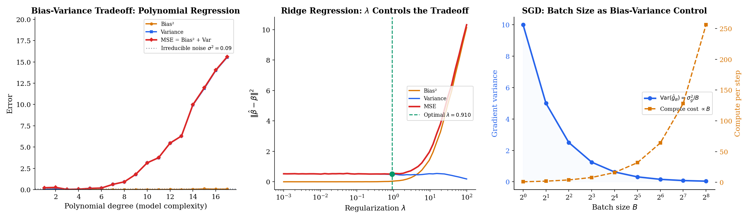
The derivation is the same add-and-subtract trick from Theorem 3, applied to instead of , with one extra term for the noise at the new test point. For a polynomial of degree fit by least squares:
- Small : is too inflexible to track ; bias is large; variance is small.
- Large : overfits to the training sample; bias is small; variance is large.
- Optimal : minimizes the sum Bias² + Variance. The irreducible noise is a floor you cannot beat without changing the problem.
This is the bias-variance picture that appears in every ML textbook — Hastie, Tibshirani & Friedman (Elements of Statistical Learning, Chapter 2.9) is the canonical reference — and it is an exact application of Theorem 3. The only difference from the scalar case is that is the “estimator” and is the “parameter” — everything else is the same decomposition.
Ridge regression (Example 12) adds to the least-squares objective, producing an estimator that is biased toward zero but has smaller variance. The MSE of the ridge predictor at a test point decomposes as before, with the -dependent tradeoff:
Bias² is monotonically increasing in (more shrinkage, more distortion of the target). Variance is monotonically decreasing in (more shrinkage, less sensitivity to the training set). The sum has a minimum at some that depends on and ; cross-validation estimates without knowing either.
The reason this works is Stein’s theorem in disguise. Shrinking OLS toward zero is a James–Stein-type operation — each coefficient gets pulled a little closer to the origin — and when the true signal is concentrated or sparse, the bias introduced is small compared with the variance reduction. In high dimensions ( but effectively for any real ML problem), the effect is pronounced: deep neural nets with L2 weight decay are the modern industrial version of this phenomenon.
Stochastic gradient descent replaces the full-batch gradient with a mini-batch estimate
where is a random subset of size . The mini-batch gradient is unbiased ( when the batch is a uniformly random sample) but has variance that scales as , where is the per-example gradient variance. This is Theorem 2 restated for the gradient estimator.
The bias-variance tradeoff in SGD is between per-step noise (small , high variance, small per-step compute) and per-step efficiency (large , low variance, large per-step compute, diminishing returns per step). Typical ML lore:
- For a fixed compute budget, the optimal batch size balances the two — larger is not always better.
- The learning rate should roughly scale linearly with : determines the per-step signal-to-noise ratio, and noise scales as while step size scales as .
- Very small batches (, pure SGD) have high variance but frequent updates — stochasticity can even help escape saddle points, a benefit absent from full-batch gradient descent.
All of this is rigorous point estimation. The “estimator” is ; the “parameter” is ; the MSE decomposes as ; and the compute cost scales linearly with . The modern deep-learning zoo of optimizers — Adam, AdamW, LAMB, Lion — are all attempts to control this MSE more cleverly, by rescaling, momentum, or variance-adaptive step sizes.
13.10 Summary
An estimator is a random variable. Its sampling distribution is the object to analyze. We have built the complete evaluation framework:
- Bias is the mean offset . Zero bias is called unbiased.
- Variance (equivalently, standard error squared) is the spread of the sampling distribution.
- MSE combines them: (Theorem 3, the central identity).
- Consistency is the guarantee that as — a consequence of the LLN.
- Asymptotic normality is the guarantee that — a consequence of the CLT.
- Fisher information is the expected curvature of the log-likelihood — how much information one observation carries about .
- Cramér–Rao bound: for every unbiased estimator. Estimators achieving the bound are efficient.
- Admissibility and minimax give global criteria for estimator comparison. The James–Stein theorem shows the sample mean is inadmissible in dimensions — shrinkage strictly improves total MSE.
The cheat sheet for every downstream topic:
| Property | Formula | Analog for ML |
|---|---|---|
| Bias | Model mis-specification / underfitting | |
| Variance | Sensitivity to training set / overfitting | |
| MSE | Bias² + Variance | Prediction error at a fixed point |
| Consistency | Convergence of training procedure | |
| Asymptotic variance | Rate of convergence, confidence interval width | |
| Fisher information | Curvature of the loss — optimization landscape | |
| CRLB | Information-theoretic lower bound on MSE | |
| Efficiency | Var / CRLB | Fraction of information the estimator extracts |
The arc of Track 4 is to apply this framework to specific estimation methods. Maximum Likelihood Estimation defines as the root of the score equation ; consistency, asymptotic normality, and asymptotic efficiency of the MLE are consequences of the LLN, CLT, and CRLB framework developed here. Method of Moments applies bias, MSE, and consistency to moment-matching estimators, comparing their efficiency to the MLE benchmark. Sufficient Statistics uses Fisher information and the CRLB to prove Rao–Blackwell and Lehmann–Scheffé theorems, thereby establishing the theory of UMVUE.
Beyond Track 4, every downstream topic in formalStatistics uses this vocabulary. Hypothesis Testing builds test statistics that are estimators; their null and alternative distributions are the consistency and asymptotic-normality statements we have just proved. The z-test applies the CLT to a standardized ; the t-test uses Basu’s theorem to give a clean distribution; the Wald, score, and likelihood-ratio tests are all -asymptotic consequences of Thm 14.3’s asymptotic-normality result. Confidence Intervals invert asymptotic-normality: a CI is an interval of the form . Linear Regression applies Gauss–Markov efficiency to OLS, which is the CRLB for Normal-error linear models; regularization and shrinkage apply Stein’s phenomenon. The Bootstrap gives empirical analogs of the sampling distribution when closed-form asymptotics are unavailable. Across formalML, the bias-variance tradeoff organizes regularization, ensembling, transfer learning, and hyperparameter tuning — the daily tools of every machine-learning practitioner.
The reader who has made it to here has the complete point-estimation toolkit: what an estimator is (§13.1), how to measure its error (§13.2–13.4), what happens as data accumulates (§13.5–13.6), how good an estimator can possibly be (§13.7), and when the “natural” choice can be uniformly beaten (§13.8). This is the foundation on which all of classical and modern statistical inference is built.
References
- Casella, G., & Berger, R. L. (2002). Statistical Inference (2nd ed.). Duxbury.
- Billingsley, P. (2012). Probability and Measure (Anniversary ed.). Wiley.
- Wasserman, L. (2004). All of Statistics. Springer.
- Lehmann, E. L., & Casella, G. (1998). Theory of Point Estimation (2nd ed.). Springer.
- Bickel, P. J., & Doksum, K. A. (2015). Mathematical Statistics: Basic Ideas and Selected Topics (2nd ed.). CRC Press.
- Hastie, T., Tibshirani, R., & Friedman, J. (2009). The Elements of Statistical Learning (2nd ed.). Springer.
- Stein, C. (1956). Inadmissibility of the Usual Estimator for the Mean of a Multivariate Normal Distribution. Proceedings of the Third Berkeley Symposium on Mathematical Statistics and Probability, 1, 197–206.
- Bishop, C. M. (2006). Pattern Recognition and Machine Learning. Springer.