Law of Large Numbers
From sample means to population truth — the weak law, the strong law, and why Monte Carlo works.
10.1 Why “In Probability” Isn’t Enough
Topic 9 ended with a promise. We proved that the sample mean converges to the population mean in probability — meaning that for any tolerance , the probability of deviating from by more than goes to zero as grows. That was Theorem 9.1, and its proof was three lines: compute the variance of , apply Chebyshev’s inequality, watch the bound vanish.
But convergence in probability is a statement about individual time slices. It says: “at time , the probability of a bad deviation is small.” It does not say that the sample path — the actual sequence of values that you observe when you run your simulation or collect your data — eventually settles down and stays near . A sequence can converge in probability without any single realization converging at all (recall the typewriter sequence from Topic 9, Section 9.7).
This distinction matters enormously in practice. When you run a Monte Carlo simulation to estimate , you run one simulation. You don’t generate infinitely many parallel universes and check that the fraction of bad outcomes is shrinking — you generate a single sequence of samples and compute a single running average. You need to know that this particular running average converges to the truth. That’s almost sure convergence: .
The same goes for stochastic gradient descent. You run one training trajectory. Polyak averaging — taking the running mean of the iterates — needs almost sure convergence of the running mean to guarantee that your single training run finds the optimum. And when you evaluate a model’s performance on a test set, the empirical risk is a sample mean. The Strong Law says this single empirical risk converges to the true risk for each fixed . The Glivenko—Cantelli theorem (Section 10.7) says something even stronger: the convergence is uniform over all thresholds — or, with the right generalization, over all simultaneously.
This topic traces the full arc from the weak law to the strong law. We start where Topic 9 left off — the Chebyshev-based WLLN for finite-variance iid sequences — and progressively generalize in two directions:
-
Relaxing assumptions (Sections 10.2—10.4): We drop the “identically distributed” requirement (uncorrelated WLLN), then drop the finite-variance requirement entirely (Khintchine’s WLLN under finite mean alone).
-
Strengthening the conclusion (Sections 10.5—10.7): We upgrade from convergence in probability to almost sure convergence (SLLN via Etemadi’s proof), then from pointwise to uniform convergence (Glivenko—Cantelli).
The bridge between these two directions is Kolmogorov’s maximal inequality (Section 10.5) — a result that controls the running maximum of partial sums with the same bound as Chebyshev uses for the terminal value. It is the technical engine that powers the SLLN proof.
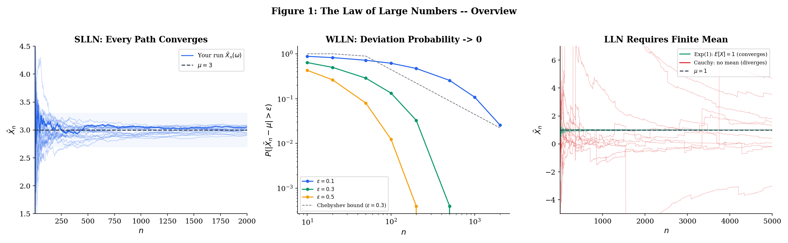
To make the distinction between the weak and strong laws concrete, consider the following analogy. Imagine you are tracking a sequence of fair coin flips, computing the running proportion of heads .
-
WLLN: For any fixed tolerance , as . If you could peek at the proportion at a single, very large time step, you’d very likely see something close to . But this says nothing about what happens if you watch the proportion evolve over time.
-
SLLN: With probability 1, the entire trajectory converges to . The running proportion settles down and stays near forever — not just at one particular time, but eventually at all times simultaneously.
The WLLN is like saying “most photos of the sequence look good.” The SLLN is like saying “the whole movie has a happy ending.” For a single run of an experiment, a simulation, or a training procedure, you are watching the movie, not snapshots — so the SLLN is the result you need.
This distinction is especially important in settings where you cannot re-run the experiment: a clinical trial with a fixed patient cohort, a one-time A/B test in production, a training run of a large language model that costs millions of dollars. You get one trajectory. The SLLN says that one trajectory is enough.
Here is the roadmap:
| Section | Result | What it says |
|---|---|---|
| 10.2 | WLLN (Chebyshev) | iid, implies |
| 10.3 | WLLN (uncorrelated) | Uncorrelated, implies |
| 10.4 | WLLN (Khintchine) | iid, implies |
| 10.5 | Kolmogorov’s maximal inequality | |
| 10.6 | SLLN (Etemadi) | Pairwise iid, implies |
| 10.7 | Glivenko—Cantelli | |
| 10.8 | Convergence rates | Chebyshev (), Hoeffding (), LIL () |
| 10.9 | ML connections | Monte Carlo, SGD/Polyak, ERM, and Glivenko—Cantelli in practice |
The first seven results are fully proved in this topic. Theorems 10.7 and 10.8 are stated without proof — the former is proved in Topic 12 (Large Deviations & Tail Bounds) as Theorem 12.3, the latter is a deep result requiring tools beyond our current scope.
10.2 WLLN for iid with Finite Variance
We begin by restating the result from Topic 9 that is our starting point. This is Theorem 9.1 transplanted into its permanent home.
Let be iid with and . Then
That is, for every , as .
The proof is recorded in Topic 9, Section 9.2: compute , apply Chebyshev’s inequality to get , and observe that the right-hand side vanishes. We do not reproduce it here — the reader should revisit the three-line argument in Topic 9 if needed.
What matters now is where this result falls short and what it leaves on the table. It requires two assumptions:
-
Identically distributed. The must all follow the same distribution — same mean, same variance, same everything. This rules out many practical settings where the noise level changes over time (heteroscedastic data) or the observations come from different subpopulations.
-
Finite variance. The variance must be finite. This excludes heavy-tailed distributions like the Student’s with degrees of freedom, the Pareto with shape , and certain financial return models where extreme events dominate.
Both assumptions are stronger than necessary. The next two sections relax them, one at a time: Section 10.3 drops “identically distributed” (replacing it with the weaker condition “uncorrelated”), and Section 10.4 drops “finite variance” entirely (requiring only a finite mean). Sections 10.5 and 10.6 then attack the second front: upgrading the conclusion from convergence in probability to almost sure convergence.
The sample mean is the simplest estimator of the population mean , and the WLLN says it is consistent: . In statistics, consistency is the bare minimum we demand of any estimator — with enough data, the estimate should converge to the truth in probability. An inconsistent estimator is fundamentally unreliable: no amount of data will make it accurate.
Every consistent estimator is, at its core, a law-of-large-numbers statement. The sample variance converges to the population variance — this is the LLN applied to the squared deviations. The empirical CDF converges to the true CDF (Section 10.7). The maximum likelihood estimator converges to the true parameter under regularity conditions — a fact whose proof uses the LLN applied to the log-likelihood.
Conversely, an estimator’s inconsistency is typically diagnosed by showing the LLN fails to apply — either because the estimator is not a sample mean (or a sufficiently well-behaved function of sample means), or because the underlying variables lack the required moment conditions.
Point Estimation & Bias-Variance formalizes this connection: an estimator is consistent if and only if it satisfies a suitable LLN — and the strength of the LLN (weak or strong) determines the strength of the consistency (convergence in probability or almost sure).
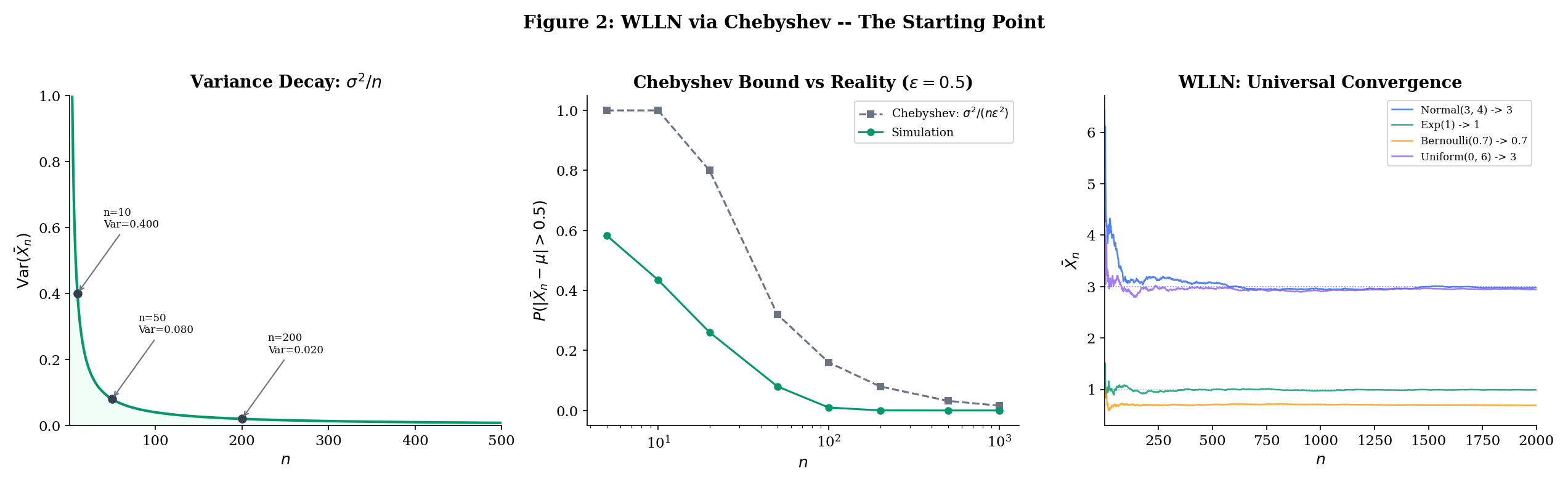
Before proceeding, it is worth noting the quantitative content of Theorem 10.1. The Chebyshev bound is not just an existence statement — it gives an explicit bound on how close is to for each . For example, if (so , ) and we want , we need , giving . This is a conservative bound — we will see in Section 10.8 that Hoeffding’s inequality gives much tighter sample-size requirements for bounded variables — but it has the virtue of requiring only the mean and variance, not the full distributional form.
It is also worth noting that the bound is distribution-free in the following sense: it holds for any distribution with mean and variance , no matter what the higher moments look like. Whether the are Normal, Uniform, Exponential, or any other distribution with finite variance, the same bound applies. This universality is both a strength (the result is extremely general — it works for any distribution with finite variance, from the Uniform to the Exponential to the chi-squared) and a weakness (the bound cannot exploit distributional structure to give tighter guarantees). Section 10.8 presents Hoeffding’s inequality, which gives exponentially better bounds by exploiting the additional assumption that the variables are bounded.
10.3 WLLN for Uncorrelated Sequences
The Chebyshev-based proof of Theorem 10.1 used two properties of the : they are identically distributed (so all means and variances are equal) and independent (so the variance of the sum is the sum of the variances). Let us examine exactly where each property entered.
The “identically distributed” assumption was used to conclude and . Without it, the mean of is (which may change with ) and the variance is (which depends on the individual variances).
The “independent” assumption was used only to show that — that is, to kill the cross-terms in . For this, independence is overkill — we only need the cross-terms to vanish. That is, we only need the to be uncorrelated.
This is a meaningful generalization. In many applied settings, variables are uncorrelated but not independent:
- In a designed experiment with orthogonal contrasts, the contrast variables are uncorrelated by construction but may not be independent (because they are all functions of the same underlying data).
- In time series analysis, residuals from a correctly specified linear model are uncorrelated (by the Gauss—Markov theorem) but not necessarily independent — the joint distribution may have higher-order dependencies.
- In random matrix theory, the entries of a Wigner matrix are uncorrelated (by the symmetric distribution assumption) but the eigenvalues are not independent.
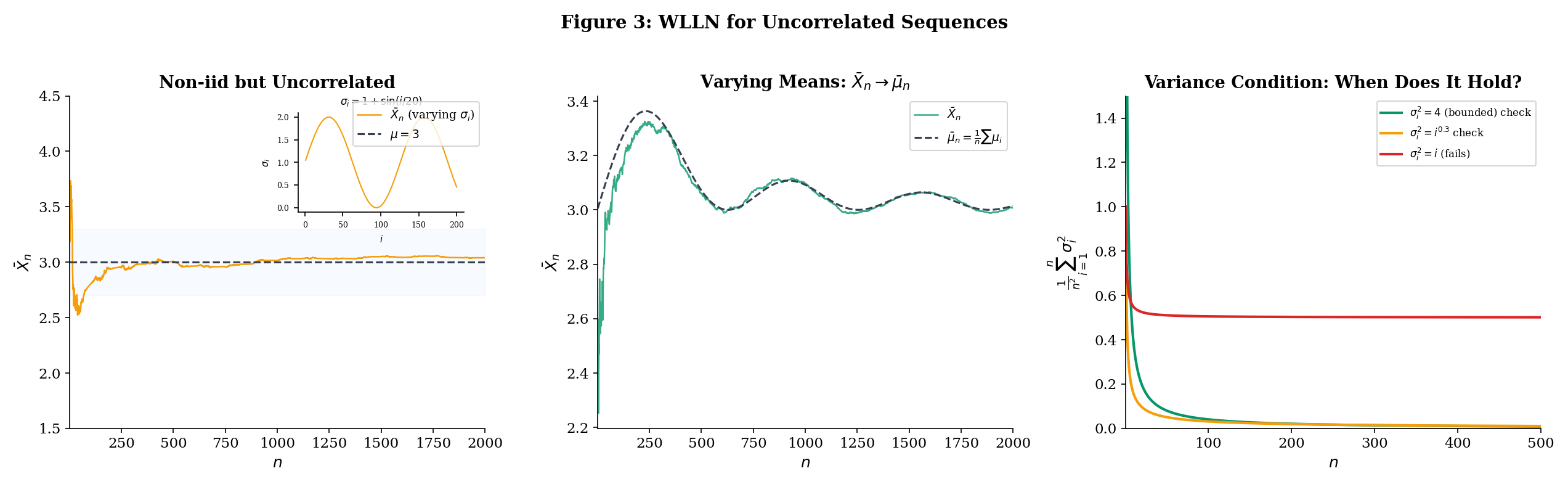
Furthermore, if the variables are not identically distributed, the sample mean may not converge to a single value — instead, it tracks the running average of the individual means . The theorem says the deviation converges to zero — the sample mean stays close to the running population mean.
Let be uncorrelated random variables (not necessarily identically distributed) with and . Define the average mean . If
then .
Proof [show]
We apply Chebyshev’s inequality to . First, note that .
For the variance, since the are uncorrelated:
The cross-terms vanish because for — this is exactly where the uncorrelated assumption enters. Independence would also give this, but uncorrelatedness is strictly weaker: two random variables can be uncorrelated without being independent (e.g., and when is symmetric about zero).
By Chebyshev’s inequality (Expectation & Moments, Theorem 12):
By hypothesis, , so the right-hand side goes to zero for every . Therefore .
The structure of the proof is identical to Theorem 10.1 — compute the variance, apply Chebyshev, watch it vanish — but the generalization is significant. We no longer require the to have the same distribution, or even to be independent. The only structural requirement is that they are uncorrelated: for . This is strictly weaker than independence (independent variables are uncorrelated, but not conversely — recall the examples from Topic 8 — Multivariate Distributions).
The condition is a Cesaro-type condition on the variances: it says the average variance doesn’t grow too fast. The most common sufficient condition is that the variances are uniformly bounded.
If the variances are uniformly bounded — for all and some constant — then
and the WLLN (Theorem 10.2) applies. In particular, if the are additionally identically distributed with common mean , then for all and we recover .
An online learning platform collects user engagement scores that measure how long (in minutes) a user spends on a task. The scores have a common population mean minutes (the true average engagement), but the variance changes over time as the platform adjusts its recommendation algorithm: .
The variances oscillate between 0.5 and 1.5 — some cohorts of users are more homogeneous than others — so they are uniformly bounded by . By Corollary 10.1, the running mean of the engagement scores converges in probability to minutes, despite the non-identical distributions. The platform can trust its running average even though the noise level fluctuates.
This is a common situation in practice: data collected over time rarely has constant variance (the phenomenon is called heteroscedasticity — literally, “different scatter”). Theorem 10.2 says the WLLN still holds as long as the variances don’t grow too fast. The Cesaro condition allows the variances to oscillate, to have isolated spikes, or even to grow slowly — as long as their running sum grows slower than .
The uncorrelated condition is also natural in many applications. If users are sampled independently, their scores are certainly uncorrelated (since independence implies uncorrelatedness), even if the measurement process changes over time.
Now consider the opposite scenario: the variance grows with time — say , perhaps because measurement noise increases as the platform scales or because the user population becomes more diverse. Then:
This does not go to zero, so the Chebyshev-based WLLN does not apply. The running mean may not converge — the growing variance can overwhelm the averaging effect. Note that the WLLN might still hold via a different proof technique (Theorem 10.2 gives a sufficient condition, not a necessary one), but the Chebyshev approach gives no guarantee.
This distinction matters when designing experiments or data collection systems: if you anticipate that measurement noise grows over time, you cannot blithely trust the running average — you may need to downweight older, noisier observations, or cap the noise via trimming.
10.4 Khintchine’s WLLN
Theorems 10.1 and 10.2 both require finite variance. Is this necessary? The answer, remarkably, is no. For iid sequences, finite mean alone suffices.
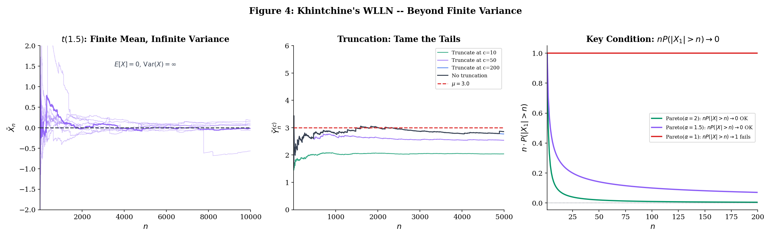
Why should we care about distributions with finite mean but infinite variance? Because they arise naturally in practice. The distribution of insurance claim sizes, financial returns, city populations, and many other real-world quantities have heavy tails — their probability of extreme values decays slowly enough that the variance is infinite, even though the mean exists. The Pareto distribution with shape parameter is the canonical example: but . If the WLLN required finite variance, we could not guarantee that sample means converge for these distributions.
Khintchine’s theorem — arguably the “right” version of the WLLN — identifies the minimal condition: .
The proof cannot use Chebyshev’s inequality (which requires a finite second moment), so we need a different technique: truncation. The idea is to clip the random variables to make their variance finite, apply the finite-variance WLLN to the clipped version, and then show that the clipping error vanishes. This is our first encounter with the truncation technique, which will reappear in the SLLN proof (Section 10.6).
The strategy has three phases, which we will see again and again in probability:
- Approximate: Replace the original variables with well-behaved versions .
- Solve the easy problem: Prove the theorem for using standard tools (Chebyshev).
- Control the error: Show that the difference between and is negligible.
Let be iid with (finite mean), but possibly . Then
Proof [show]
The key idea: even when the variance is infinite, we can truncate the random variables to make the variance finite, apply the finite-variance WLLN to the truncated version, and then show the truncation error vanishes. The truncation threshold grows with the sample size — a clever coupling that makes everything work.
Step 1: Truncate. Define — the version of where values exceeding in absolute value are zeroed out. Note that the truncation threshold is (the sample size), not a fixed constant. This is essential: as grows, the truncation becomes less aggressive, eventually including every finite value.
Step 2: Show the truncation error is negligible. We need . The events are the events where truncation changes the -th variable. By the union bound:
where the last equality uses the identical distribution of the . We claim .
To see this, note that . We need a sharper bound than Markov’s inequality (which gives , a bound that does not vanish). Instead, observe that (since on the event ). Therefore:
Since pointwise as (for every outcome where , which is almost every outcome since ), and with , the dominated convergence theorem ( formalCalculus: The Riemann Integral & FTC ) gives:
Therefore , which means .
Step 3: Center the truncated variables. Let . By DCT (since pointwise and ):
Step 4: Apply the finite-variance WLLN to the truncated variables. The are iid (as functions of iid ) with , so . But we need , which requires . The crude bound gives , which does not vanish. We need a sharper estimate.
Since implies , we have:
The right side converges to by DCT. But we need it to show , not just that it’s bounded. Let us be more careful. We have:
For each fixed , as (the numerator is fixed while the denominator grows). The integrand is bounded by (using on the indicator). Since , DCT gives:
Therefore , and by Chebyshev’s inequality:
Step 5: Combine. We have three convergence statements:
- (Step 2)
- (Step 4)
- (Step 3, deterministic convergence)
Therefore:
which gives .
The truncation technique is a workhorse of probability theory. The pattern — replace a badly-behaved random variable with a well-behaved approximation, handle the approximation with standard tools, then bound the approximation error — appears throughout convergence theory. We will see it again in the SLLN proof (Section 10.6), where the truncation threshold is rather than . The CLT proof uses the same idea with characteristic functions. In empirical process theory, truncation is the first step in proving maximal inequalities for unbounded function classes.
The key insight is that the truncation threshold grows with . A fixed threshold would introduce a permanent bias (the truncated mean is generally not equal to ). By letting the threshold grow, the bias vanishes — the truncated mean converges to the true mean — while the variance is still controlled because the growth rate of the threshold is calibrated to the sample size.
Let us also highlight where the dominated convergence theorem entered, because its role is subtle. The DCT was used in three places:
- Step 2: To show — the tail expectation vanishes. The dominating function is itself.
- Step 3: To show — the truncated mean converges to the true mean.
- Step 4: To show — the key variance bound. Here the dominating function is , and the pointwise convergence uses the fact that the numerator is a fixed number while the denominator grows.
Each application follows the same pattern: the integrand converges pointwise and is dominated by an integrable function, so the integral converges. The DCT is the workhorse of truncation arguments throughout probability theory. See formalCalculus: The Riemann Integral & FTC for the full statement and proof.
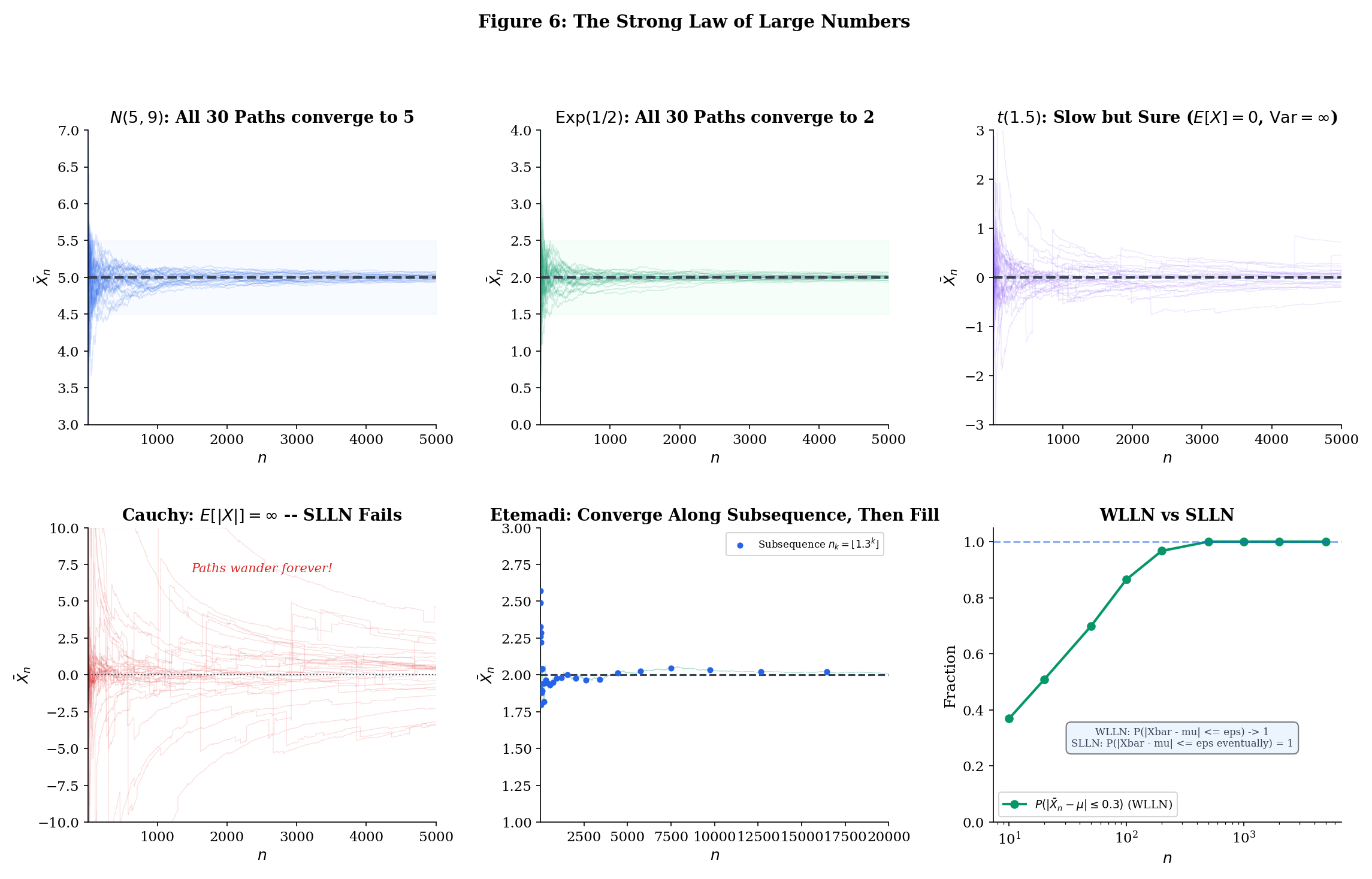
The Student’s distribution with degrees of freedom has (the mean exists when ) but (the variance is infinite when ). The Chebyshev-based WLLN (Theorem 10.1) does not apply — we cannot even compute the bound because .
Khintchine’s theorem (Theorem 10.3) guarantees regardless. But the convergence is painfully slow — much slower than for distributions with finite variance.
Why? The heavy tails of the produce occasional extreme values — observations 10, 100, or even 1000 times larger than typical — that jerk the running mean away from zero. These outliers become rarer as grows (the truncation argument ensures this), but their impact on the average is large enough to cause visible fluctuations even at sample sizes where a Normal or Exponential running mean would have long since settled down. The Chebyshev rate is not available (because ), and the effective convergence rate is slower than .
How slow is “painfully slow”? For (which has ), the Chebyshev bound gives . At , this is at most 1%. For , we cannot even write down a Chebyshev bound because the variance is infinite. Empirically, the sample mean of observations from still shows fluctuations of order 0.1 or more with noticeable probability — a tenfold degradation compared to the Normal.
The interactive WLLN Explorer (above) lets you compare the convergence speed of the sample mean for different distributions. Try setting the distribution to and comparing with — both have mean zero, but the convergence to zero is visibly rougher for the .
Khintchine’s original proof used characteristic functions rather than truncation. The characteristic function always exists (even when moments are infinite), and for iid with mean :
Since near (this expansion requires only ), we get , which is the characteristic function of the constant . By Levy’s continuity theorem, , and convergence in distribution to a constant is equivalent to convergence in probability.
This approach is more elegant but requires Fourier analysis (specifically, the expansion for small, which holds whenever ). The truncation proof above uses only tools we have already developed: Chebyshev’s inequality and the dominated convergence theorem. The characteristic function proof has the advantage of immediately giving convergence in distribution, which implies convergence in probability to a constant — but the truncation proof is more transparent about where the finite-mean assumption is used.
10.5 Kolmogorov’s Maximal Inequality
The three WLLN results (Theorems 10.1—10.3) all establish convergence in probability: . To upgrade to almost sure convergence, we need to control the entire path of partial sums, not just the terminal value . This is a fundamentally harder problem. Convergence in probability is a statement about each fixed time ; almost sure convergence is a statement about the entire infinite trajectory simultaneously.
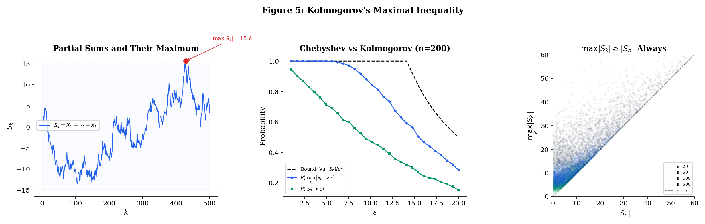
The key question is: how large can the partial sums get along the way? Chebyshev’s inequality controls — the probability that the final partial sum is large. But the partial sums might wander far from zero at intermediate times and then return. A random walk, for instance, typically reaches a maximum that is much larger than its terminal value. For the SLLN, we need to control — the probability that any partial sum along the way is large.
You might guess that controlling the maximum would cost a factor of (by the union bound: , and each term is bounded by Chebyshev). Kolmogorov’s maximal inequality does dramatically better: the bound is the same as Chebyshev’s for the terminal value alone. Controlling the running maximum costs nothing extra. This “free upgrade” is the mathematical reason why the SLLN proof works — it converts Chebyshev-type bounds (which give convergence in probability) into bounds on the running maximum (which, via Borel—Cantelli, give almost sure convergence).
Let be independent random variables with and . Define partial sums . Then for any :
Proof [show]
The right-hand side is identical to the Chebyshev bound for . The fact that controlling the maximum over all gives the same bound is what makes this inequality powerful. The proof uses a clever decomposition based on the first time the partial sum exceeds the threshold.
The stopping time idea. Define the event — the event that the partial sum first exceeds in absolute value at time . These events are disjoint (the first exceedance can only happen once), and their union is the event that the maximum exceeds :
Decompose . We split according to whether the maximum exceeds :
The second term is non-negative (it is the expectation of a non-negative random variable), so:
Key step: Expand on each . On the event , we decompose the final partial sum into the value at the first exceedance time plus the remaining increments:
Since , we have . Taking expectations restricted to :
Now comes the crucial observation. The random variable is a function of alone (because and the event depend only on the first variables). The random variable depends only on . By independence of the , these two quantities are independent. Therefore:
Since for all :
So the cross-term vanishes: . This gives:
On the event , we have , so . Therefore:
Summing over . Combining the chain of inequalities:
Rearranging:
which is the claimed bound.
The proof is entirely elementary — no advanced machinery, just a decomposition based on the first exceedance time and the observation that independence kills the cross-term. This is the same “orthogonality” trick that makes the variance of a sum equal the sum of the variances, applied more carefully.
Let us pause to appreciate why this result is surprising. A naive approach to controlling would use the union bound:
This gives a bound that grows like — a factor of worse than Kolmogorov’s inequality. The stopping-time decomposition avoids this factor-of- loss by exploiting the independence structure: the future increments are independent of the past, so the cross-term vanishes. Without independence, the best we could do is the union bound.
This factor-of- savings is exactly what allows the Borel—Cantelli argument in the SLLN proof to succeed: the summable probability bounds from Kolmogorov’s inequality, summed over the geometric subsequence, converge — whereas the union-bound version would diverge.
Let be iid , so is a random walk. The terminal value has the same distribution as for , with typical magnitude . But the running maximum is typically larger — the path might wander far from zero at some intermediate time and then return.
The reflection principle from probability theory gives (slightly larger than by a constant factor). Yet Kolmogorov’s inequality tells us that the tail probability satisfies the same bound as : both are at most . Controlling the maximum path is no harder than controlling the endpoint, at least in terms of the Chebyshev-type bound.
For steps, a typical random walk has (since ) but or more. The Kolmogorov bound says — the same bound we would get from Chebyshev for .
The interactive explorer below shows sample paths of the random walk with both (the endpoint) and (the running maximum) highlighted. Notice how the running maximum can be substantially larger than the endpoint, yet the Kolmogorov bound still holds.
Kolmogorov’s maximal inequality is a special case of Doob’s maximal inequality for submartingales. When , the partial sums form a martingale (the conditional expectation of given equals ), and is a submartingale. Doob’s inequality gives the same bound in greater generality: for any non-negative submartingale ,
Applied to and , this recovers Kolmogorov’s inequality. We do not need the full martingale theory here — the stopping-time decomposition above is elementary and self-contained — but the reader should be aware that the maximal inequality is part of a much richer theory.
10.6 The Strong Law of Large Numbers
We are now ready for the main event. The Strong Law of Large Numbers says that the sample mean converges to the population mean almost surely — not just in probability. Recall from Topic 9 that almost sure convergence is strictly stronger than convergence in probability: it says that the probability of the event “the sample path converges to ” is 1, not merely that the probability of being far from at any particular time goes to zero.
This distinction is not academic. When you run a Monte Carlo simulation to estimate an integral, you run one simulation and observe one trajectory of running averages. You need that trajectory to converge — not just that most trajectories converge, but that yours does. The SLLN says: with probability 1, yours does. When you train a neural network with SGD, you run one training trajectory. The SLLN (and its martingale generalizations) says that trajectory converges. When you evaluate a model on a test set, you compute one empirical risk. The SLLN says it converges to the true risk. Almost sure convergence is what makes single-run inference valid.
We follow the proof of Etemadi (1981), which is remarkable in two respects. First, it requires only pairwise independence — not the full mutual independence that most proofs assume. Second, it is genuinely elementary: the only tools are the Kolmogorov maximal inequality (Theorem 10.4), the first Borel—Cantelli lemma (from Modes of Convergence), and the dominated convergence theorem ( formalCalculus: The Riemann Integral & FTC ). No characteristic functions, no martingale theory, no measure-theoretic heavy machinery. Etemadi’s original paper (1981) is three pages long — one of the shortest proofs of a fundamental theorem in all of probability. Before Etemadi, the standard proof (due to Kolmogorov) required full mutual independence and used the Kolmogorov three-series theorem, which itself requires significant machinery. Etemadi’s contribution was to show that pairwise independence suffices, using only the tools we have developed here.
Let be pairwise independent, identically distributed random variables with . Then
That is, .
Proof [show]
We follow Etemadi’s 1981 proof, which is remarkable for requiring only pairwise independence (not full independence). The argument has three stages: reduce to non-negative random variables, prove convergence along a geometric subsequence using truncation and Borel—Cantelli, then fill in the gaps between subsequence terms using monotonicity.
Stage 1: Reduce to non-negative random variables.
Write where and . Since , both and are finite (because and ). The sequences and are each pairwise independent and identically distributed with finite mean.
If we prove the SLLN for non-negative random variables, then:
Subtracting (the difference of two a.s. convergent sequences converges a.s., since a.s. convergence is preserved under finite linear combinations) gives:
So without loss of generality, assume for the remainder of the proof. This assumption buys us something crucial: when , the partial sums are non-decreasing in . This monotonicity is what makes Stage 3 work.
Stage 2: Truncate and prove convergence along a geometric subsequence.
Fix an integer (the standard choice is , but any integer works). Define the geometric subsequence for The key insight is to first establish convergence along this sparse subsequence — which is easier because the gaps between terms grow geometrically, making certain series converge — and then fill in the gaps using monotonicity.
The plan: prove almost surely (the hard part, Steps 2a—2e), then show for all between consecutive subsequence terms (Stage 3, using monotonicity from Stage 1).
Step 2a: Truncation. Define truncated variables . Since , the truncation simply caps values exceeding at zero: if , then ; if , then . Note that the truncation threshold for the -th variable is itself (not , as in the Khintchine proof). This is a different calibration — each variable gets its own threshold, growing with its index. Let denote the centered truncated variables.
Step 2b: The truncation error vanishes almost surely. We need to show that for all but finitely many , with probability 1. Consider the “bad” events — the events where the -th observation exceeds the -th truncation threshold. Since the are identically distributed:
The inequality follows from the tail-sum formula for expectation of non-negative integer-valued random variables, or more precisely from comparing the sum to the integral:
By the first Borel—Cantelli lemma ( formalCalculus: Series Convergence ): since , the probability that occurs for infinitely many is zero. In other words, with probability 1, for all but finitely many . For those finitely many exceptions, — but a finite number of mismatches does not affect the asymptotic behavior of a sample mean. Therefore, the sample means of and have the same a.s. limit (if either has one).
Step 2c: The variance series converges. For Borel—Cantelli to work in Step 2d, we need a summable series of probability bounds. This in turn requires that the variances of the truncated variables, when summed with appropriate weights, converge. Specifically, we need . Since (the variance is at most the second moment), it suffices to show :
We interchange the sum and expectation using Tonelli’s theorem (both are non-negative):
For (or more precisely, ), the inner sum satisfies:
(by comparison with the integral ). Therefore , giving:
This is where (equivalently since ) is used — and it is the only place in the proof where the finite-mean assumption enters in an essential way. If , the series would diverge, and the entire argument would collapse.
Step 2d: Apply Kolmogorov’s maximal inequality along the subsequence. This is the step where Kolmogorov’s inequality (Theorem 10.4) enters. For each , consider the centered truncated partial sums . The are pairwise independent (since each is a function of alone, and the are pairwise independent) with . By Kolmogorov’s maximal inequality, for any :
We need of the right-hand side to converge (so Borel—Cantelli applies). Since :
Exchanging the order of summation (each appears in the inner sum for all with , i.e., ):
where is a geometric series constant (for , this is ). Since (Step 2c), the entire sum converges. This is where the geometric spacing of the subsequence is essential: with equally spaced terms (), the sum would not converge.
By the first Borel—Cantelli lemma ( formalCalculus: Series Convergence ): since , the probability that the event occurs for infinitely many is zero. That is:
In particular, taking :
Step 2e: The means of the truncated variables converge. Since by DCT ( formalCalculus: The Riemann Integral & FTC ):
(This is a Cesaro mean of a convergent sequence. By the Cesaro lemma, if , then . Here , so the Cesaro mean also converges to .)
Combining Steps 2d and 2e:
By Step 2b, for all sufficiently large (almost surely). This means the partial sums and differ by at most a finite constant (the sum of the finitely many terms where ). Dividing by , this finite difference becomes negligible. Therefore almost surely.
Stage 3: Fill in the gaps between subsequence terms.
For , we use the non-negativity of the to squeeze the sample mean. Let . Since each , the partial sums are non-decreasing: . Therefore:
The left inequality holds because (adding more non-negative terms can only increase the sum) and (dividing by a larger denominator makes the fraction smaller), so . The right inequality holds because (the sum of more terms is larger) and (dividing by a smaller denominator makes the fraction larger), so .
Now we evaluate the bounds as . The lower bound:
The upper bound:
So for every between and , the sample mean is squeezed between values converging to and .
Since is fixed, the lower bound approaches and the upper bound approaches — useful, but not the that we want. The squeeze is too loose because the ratio between consecutive subsequence terms is too large. But we can still extract the result by combining the squeeze with the WLLN.
For any :
almost surely. Now, the left-hand side and right-hand side hold for every integer . Taking does not help — the bounds get worse (the squeeze widens). But we can finesse this with the following observation.
The random variables and are both tail random variables — they depend only on the tail of the sequence. By Kolmogorov’s 0-1 law (Remark 4), each is almost surely constant: a.s. and a.s. for some deterministic constants with .
The squeeze gives and for every . This constrains and but does not pin them down. However, the WLLN (Theorem 10.3, which we proved independently) tells us . Convergence in probability to a constant implies that any almost-sure subsequential limit must equal that constant. Since and are the infimum and supremum of the subsequential limits, we must have:
Therefore almost surely.
Let us step back and appreciate the structure of Etemadi’s argument, because it is a masterclass in mathematical proof technique:
-
Stage 1 reduces to non-negative variables — a clean trick that unlocks monotonicity in Stage 3. The decomposition is standard, but its use here is strategic: monotonicity of partial sums is what lets us fill in the gaps between subsequence terms.
-
Stage 2 is the hard work, and it interleaves three ideas. Truncation () makes the variance summable — this is where is used, via the interchange-of-sum trick . Kolmogorov’s maximal inequality controls the running maximum of the centered partial sums, not just the terminal value. Borel—Cantelli converts the summable probability bounds into almost sure convergence, but only along the geometric subsequence .
-
Stage 3 fills in the gaps using the non-negativity from Stage 1. The squeeze traps every between two sequences that both converge to .
The proof requires only pairwise independence — a remarkable weakening of the usual assumption. Full mutual independence is not needed for two reasons. First, the Kolmogorov maximal inequality proof (Theorem 10.4) uses independence only to show that the future increment is independent of ; for the variance calculation , pairwise independence suffices. Second, the first Borel—Cantelli lemma ( implies ) makes no independence assumption at all — it is a purely measure-theoretic fact.
This pairwise-independence generalization is not just a mathematical curiosity. In several practical settings, observations are pairwise independent but not mutually independent:
- Sampling without replacement from a finite population: knowing that observation 1 and observation 2 take specific values tells you something about observation 3 (the population is slightly depleted), so the three are not mutually independent. But any two observations are pairwise independent (each pair is equally likely to produce any pair of values).
- Hash-based sampling: Random hash functions with pairwise independence (2-universal hash families) are widely used in streaming algorithms. The SLLN via Etemadi applies to averages computed from such samples.
Etemadi’s theorem guarantees that the SLLN still holds in all these settings.
The following proposition confirms that finite mean is not just sufficient but necessary for the SLLN.
If are iid and converges almost surely (or even in probability) to a finite limit, then .
The proof uses the converse direction of the Borel—Cantelli lemma. If , then (since , which is infinite). By the second Borel—Cantelli lemma — which applies here because the events are independent (they depend on different ‘s) — we get .
This means that with probability 1, the sequence contains infinitely many terms with . Each such term contributes at least to the sample mean (since ), and these large contributions arrive infinitely often. A careful argument shows this prevents from converging to any finite limit. The details are in Durrett (2019, Theorem 2.4.5).
The takeaway: is the exact boundary for the LLN. Below this threshold (e.g., the Cauchy with ), sample means do not converge to any finite limit. At or above this threshold, they converge almost surely to . The condition is sharp — it cannot be weakened.
The Cauchy distribution (equivalently, Student’s with degree of freedom) has density . It has no finite mean: (the integral diverges logarithmically).
Proposition 10.1 says the SLLN must fail. But something much more dramatic is true: the sample mean of iid Cauchy random variables does not converge at all. In fact, is itself Cauchy-distributed for every — with the exact same distribution as a single observation.
This follows from the Cauchy being a stable distribution: if are iid standard Cauchy, then has the same distribution as (Cauchy with scale parameter ). Dividing by gives — the averaging accomplishes nothing. No matter how large is, the sample mean is just as dispersed as a single observation.
This is not just slow convergence — it is no convergence. The sample mean carries zero information about the “center” of the Cauchy distribution, no matter how many observations you collect. The median, by contrast, does converge: the sample median of iid Cauchy observations converges to the location parameter at rate . This is a vivid illustration of why the choice of estimator matters — the sample mean is the wrong tool for heavy-tailed data.
Try setting the degrees of freedom to in the SLLN Explorer below. The sample paths wander without settling down — a striking contrast to the well-behaved convergence seen with distributions that have a finite mean. Then try (finite mean, infinite variance) to see slow but genuine convergence, and (finite variance) to see rapid convergence.
The event is a tail event: it depends only on the “tail” of the sequence. More precisely, for any finite , changing does not affect whether converges as — the convergence or non-convergence is determined by the behavior of The tail -algebra captures exactly these “asymptotic” events.
Kolmogorov’s 0-1 law states: if are independent, then every event in has probability 0 or 1. There is no middle ground — you cannot have , for instance.
This means that even before proving the SLLN, we know the answer must be all-or-nothing: either or . The SLLN’s job is to determine which one. Etemadi’s proof shows that when , the answer is 1. Proposition 10.1 shows that when , the answer is 0. The 0-1 law ensures there are no other possibilities.
Other tail events include , , and . All of these have probability 0 or 1. The 0-1 law is one of the most elegant results in probability: it says that for independent sequences, every question about the “eventual behavior” has a deterministic answer — even though the individual random variables are random, the tail behavior is not.
The 0-1 law requires independence (or at least that the tail -algebra is trivial). For dependent sequences (such as Markov chains), the tail behavior can genuinely have intermediate probabilities. This is why the SLLN for Markov chains (the ergodic theorem) requires additional conditions beyond what the iid SLLN needs — specifically, irreducibility, aperiodicity, and positive recurrence (Topic 26 §26.7 Thm 5).
10.7 The Glivenko-Cantelli Theorem
The SLLN says that the sample mean converges to almost surely. But sample means are just one kind of statistic. What about the entire distribution of the data? Can we estimate the CDF of from a sample?
The natural estimator is the empirical CDF: the proportion of observations at or below each threshold . The Glivenko—Cantelli theorem says this estimator converges to the true CDF not just pointwise (which would follow immediately from the SLLN applied to indicator functions) but uniformly over all — and almost surely.
Given iid observations with common CDF , the empirical CDF (ECDF) is:
For each fixed , is the sample mean of the Bernoulli random variables , each with mean .
The ECDF is a step function that jumps by at each observation. It is itself a valid CDF (of the discrete uniform distribution that places mass on each observed value ). As a function of , it is non-decreasing and right-continuous, just like any CDF.
The ECDF is the most fundamental object in nonparametric statistics. Unlike parametric estimators (which assume the data comes from a specific family), the ECDF estimates the entire distribution without any assumptions. Every summary statistic you compute from data — the sample mean, the sample variance, the sample median, the sample quantiles — can be expressed as a functional of the ECDF. The sample mean is . The sample variance is . The sample -quantile is . The interquartile range is . In this sense, the ECDF is the “mother” of all nonparametric statistics — if the ECDF converges to the true CDF, then every continuous functional of the CDF is consistently estimated by the corresponding functional of the ECDF.
For each fixed , the SLLN immediately gives , since is the sample mean of iid Bernoulli variables with mean , and . This gives pointwise a.s. convergence — the ECDF converges to the true CDF at each individual threshold.
But pointwise convergence is not enough. If we want to use the ECDF to estimate quantiles, test distributional hypotheses, or construct confidence bands, we need convergence that holds at all simultaneously. The problem is that the pointwise SLLN gives a probability-1 set for each on which , but different ‘s may have different exceptional sets. Since ranges over the uncountable set , we cannot simply intersect the probability-1 sets (an uncountable intersection of probability-1 sets need not have probability 1).
The Glivenko—Cantelli theorem overcomes this obstacle by exploiting the monotonicity of CDFs. The key idea is that an uncountable supremum over can be bounded by a finite maximum over grid points plus a discretization error — and this works because CDFs cannot oscillate freely between grid points. The argument is an -net argument: approximate the uncountable index set by a finite grid, handle the grid points with the SLLN, and control the approximation error using monotonicity.
This is worth highlighting because the same -net technique — with different notions of “grid” and “approximation error” — is the template for all uniform convergence results in probability and statistics, from the Glivenko—Cantelli theorem to uniform laws of large numbers over function classes.
Let be iid with CDF . Then:
The empirical CDF converges to the true CDF uniformly and almost surely.
Proof [show]
The challenge is upgrading from pointwise to uniform convergence. The SLLN gives convergence at each fixed , but taking the supremum over uncountably many requires an additional argument. The key insight is that CDFs are monotone, so the supremum over all can be bounded by the maximum over finitely many grid points plus a discretization error controlled by the CDF’s own oscillation.
Step 1: Pointwise convergence via SLLN. Fix any . The random variables are iid Bernoulli — they equal 1 with probability and 0 otherwise. Their mean is and they certainly have . By the SLLN (Theorem 10.5):
This gives pointwise a.s. convergence at every , but we need uniform convergence.
Step 2: Discretize using partition points. Fix . Since is non-decreasing with and , we can choose points such that:
(We define and .) This is possible because is right-continuous — we can always refine the partition to make the jumps smaller than .
Step 3: Bound the supremum using the grid. For any , there exists such that . Since both and are non-decreasing:
For the upper bound on :
For the upper bound on :
Combining both bounds:
Taking the supremum over all :
Step 4: Apply the SLLN at finitely many points. By Step 1, for each . Since the intersection of finitely many probability-1 events has probability 1, there exists a single event with on which for all simultaneously.
On , for all sufficiently large :
Combining with the bound from Step 3: for all larger than some ,
The crucial point is that depends on (since the SLLN convergence is sample-path dependent) but not on — the same works for all simultaneously, because we reduced the uncountable supremum to a finite maximum in Step 3.
Step 5: Remove the dependence on . Steps 2—4 showed that for each fixed , there exists a probability-1 set on which eventually. But depends on (because the grid points depend on ). To get a single probability-1 set that works for all , we use a standard countable-intersection trick.
Let . This is a countable intersection of probability-1 events, so (by countable subadditivity of probability). On , for every integer , we have for all sufficiently large . Since is arbitrary:
Therefore .
The proof’s strategy — reduce an uncountable supremum to a finite maximum plus a discretization error — is a template that recurs throughout empirical process theory. The monotonicity of CDFs is what makes the discretization work: between two grid points, neither nor can oscillate freely, so the error from approximating the continuous supremum with a finite maximum is controlled by the mesh of the partition.
Notice what the proof does not require: any assumption on the distribution . The Glivenko—Cantelli theorem holds for every CDF — continuous, discrete, mixed, any distribution whatsoever. This is because the proof uses only three properties of CDFs: they are non-decreasing, they go from 0 to 1, and they have at most countably many discontinuities. The SLLN provides the pointwise convergence; monotonicity and the -net argument upgrade it to uniform convergence.
The quantity is known as the Kolmogorov—Smirnov (KS) statistic. It measures the worst-case discrepancy between the empirical and true CDFs — the maximum vertical gap between the step function and the smooth curve . The Glivenko—Cantelli theorem says a.s.; the Dvoretzky—Kiefer—Wolfowitz (DKW) inequality (stated in Example 5 below) gives exponential concentration around zero; and the Kolmogorov distribution gives the exact limiting distribution of , which is the foundation of the KS test for goodness of fit. Topic 29 §29.5 and §29.8 develop DKW with Massart’s tight constant and the asymptotic Kolmogorov distribution in full.
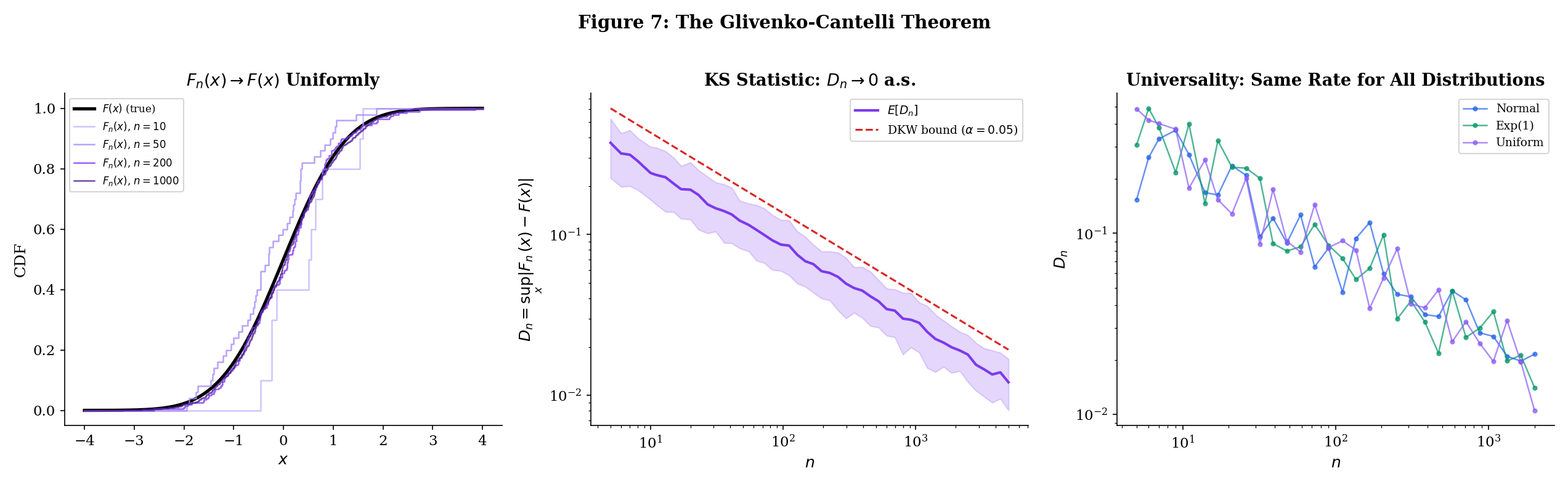
Generate observations from . The empirical CDF is a step function that approaches the smooth CDF . The Kolmogorov—Smirnov (KS) statistic is:
The Glivenko—Cantelli theorem says almost surely. But how fast? The Dvoretzky—Kiefer—Wolfowitz (DKW) inequality gives an exponential rate:
At , with high probability. At , . At , . The decay is at rate — specifically, converges in distribution to the Kolmogorov distribution (the supremum of a Brownian bridge), which is the basis of the Kolmogorov—Smirnov test for goodness of fit.
The KS test is one of the most widely used nonparametric tests: to test whether a sample comes from a particular distribution , compute and reject if it is too large (compared to the quantiles of the Kolmogorov distribution). The Glivenko—Cantelli theorem is what makes this test valid — it guarantees that under the null hypothesis , the KS statistic converges to zero, so large values of are evidence against .
The two-sample KS test compares two empirical CDFs and from potentially different distributions. The test statistic converges to by Glivenko—Cantelli applied to each sample, so the test can detect any difference between the two distributions — not just differences in mean or variance, but differences in shape, skewness, or tail behavior. This omnibus property is what makes the KS test valuable as a diagnostic tool in model validation.
In machine learning, the KS test has several applications:
- Dataset shift detection: Compare the ECDF of a feature in the training data to the ECDF in the production data. If the KS statistic is large, the distribution has shifted, and the model may need retraining.
- Model validation: After training a generative model, compare the ECDF of generated samples to the ECDF of real data. The KS statistic measures how well the model captures the true distribution.
- Feature engineering: The KS statistic between the ECDFs of a feature conditioned on different classes measures the feature’s discriminative power.
The Glivenko—Cantelli theorem guarantees that all these comparisons are meaningful: both ECDFs converge to their respective true CDFs, so the KS statistic consistently estimates the true discrepancy.
10.8 Convergence Rates
The SLLN says almost surely — but how fast? This is not just a theoretical curiosity. In practice, the convergence rate determines how many samples you need to achieve a desired accuracy. A Monte Carlo estimate with samples might be adequate if the convergence is fast, or catastrophically unreliable if it is slow. The difference between polynomial and exponential convergence rates can mean the difference between and samples for the same accuracy guarantee.
Three results give increasingly precise answers, forming a hierarchy of convergence rate statements:
- Chebyshev’s inequality — polynomial rate, weakest but most general
- Hoeffding’s inequality — exponential rate for bounded variables
- Law of the iterated logarithm — the exact a.s. oscillation envelope
The Chebyshev rate. From Theorem 10.1, . This is a polynomial decay: the probability of an -deviation decreases like . For a fixed confidence level , we need samples to guarantee . This is often pessimistic — Chebyshev uses only the mean and variance, ignoring all other information about the distribution. For bounded or sub-Gaussian variables, the true rate is much faster.
Let be independent with almost surely. Then for any :
For iid variables with :
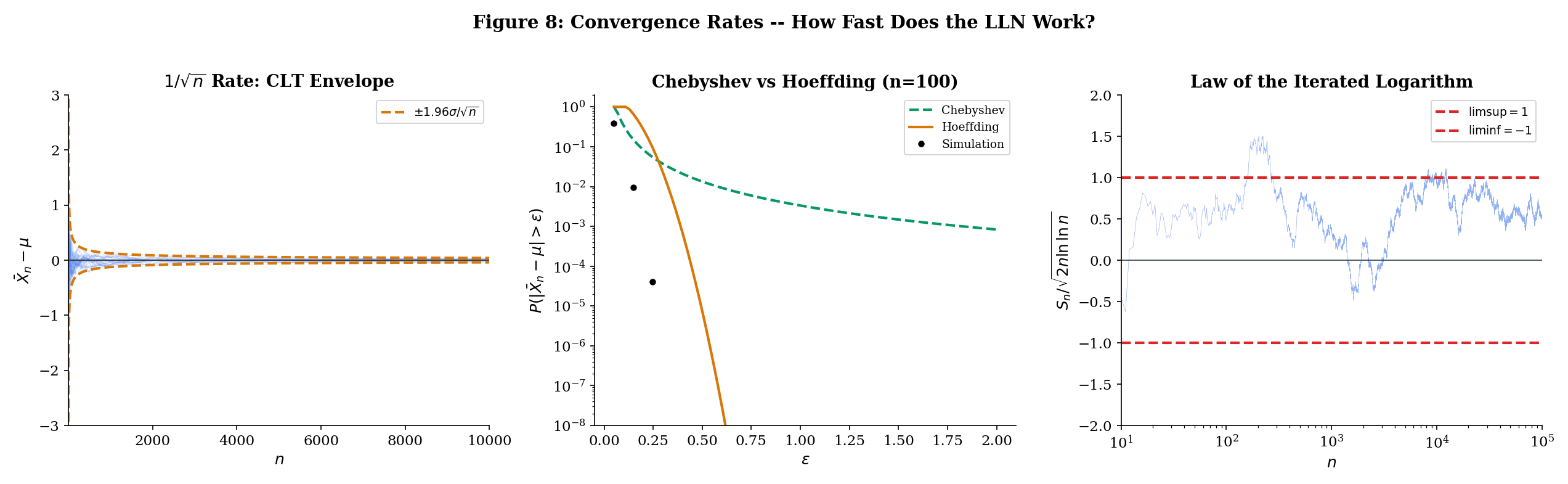
The improvement over Chebyshev is dramatic. Chebyshev gives polynomial decay: , which is . Hoeffding gives exponential decay: , which goes to zero exponentially fast in . The practical difference is enormous — it determines how many samples you need for a given confidence level. For and (so ):
| Chebyshev bound | Hoeffding bound | |
|---|---|---|
| 100 | 2.500 (useless) | 0.271 |
| 500 | 0.500 | 0.000045 |
| 1000 | 0.250 | |
| 5000 | 0.050 |
At , Chebyshev says the probability of a 0.1 deviation is at most 25%, while Hoeffding says it is at most two in a billion. At , Chebyshev gives 5% (barely useful) while Hoeffding gives (effectively zero).
The practical implication: if you need a confidence guarantee of for bounded variables, Chebyshev requires samples (at least for ). Hoeffding requires samples — nearly three times fewer. The Chebyshev bound is useless for practical sample-size calculations; the Hoeffding bound is tight enough to be actionable.
The full proof of Hoeffding’s inequality uses the Chernoff bounding technique: apply Markov’s inequality to instead of , then optimize over . The exponential transform converts additive structure (the sum of independent variables) into multiplicative structure (a product of MGFs), which is much easier to control. The boundedness assumption enters through the Hoeffding lemma, which bounds the MGF of a bounded random variable. The full development is the subject of Large Deviations & Tail Bounds — the Chernoff technique, Hoeffding’s lemma, and the complete proof are in §§12.2–12.3.
The third result tells us the exact a.s. rate at which fluctuates around .
Let be iid with and . Then almost surely:
The sample mean oscillates within the envelope and touches both boundaries infinitely often.
The LIL gives an astonishingly precise description of the a.s. behavior. The SLLN says . The LIL says exactly how it approaches zero: the fluctuations are of order , which is slightly larger than the CLT scale of (by a factor of ). The sample path oscillates within this shrinking envelope, touching the upper and lower boundaries infinitely many times — it never stays on one side permanently.
The double logarithm grows extraordinarily slowly: , , , . So the LIL envelope is only slightly wider than the CLT scale . In practice, the LIL is more of a theoretical landmark than a computational tool — it tells us that the SLLN convergence rate cannot be faster than , establishing a fundamental limit on how quickly sample means can settle down.
The proof of the LIL is deep (it uses the second Borel—Cantelli lemma and exponential tail bounds) and beyond our scope here. We state it to complete the picture of how the LLN, the CLT, and the LIL form a hierarchy of increasingly precise statements about .
Three results describe at different levels of precision:
SLLN (Theorem 10.5): almost surely. The fluctuations vanish. This is the qualitative statement — convergence happens. It answers the question: does converge?
Law of the Iterated Logarithm (Theorem 10.8): The fluctuations are exactly of order . This is the quantitative envelope — how tightly the sample path concentrates around . It answers: how closely does track ?
Central Limit Theorem: . The fluctuations at scale are approximately Normal. This is the distributional statement — the shape of the fluctuations. It answers: what do the deviations look like at any given ?
Each tells you more. The SLLN says “it converges.” The LIL says “the deviations decay like .” The CLT says “at the scale , the deviations look Gaussian.”
These are not competing statements — they complement each other. The SLLN is a pathwise result (it says something about almost every ). The LIL is also pathwise (it gives the exact a.s. oscillation). The CLT is distributional (it says what the distribution of looks like for large ). Concentration inequalities like Hoeffding (Theorem 10.7) are tail probability bounds (they say how fast decays). Large Deviations & Tail Bounds develops these exponential-rate guarantees — the most useful results for practical sample-size calculations.
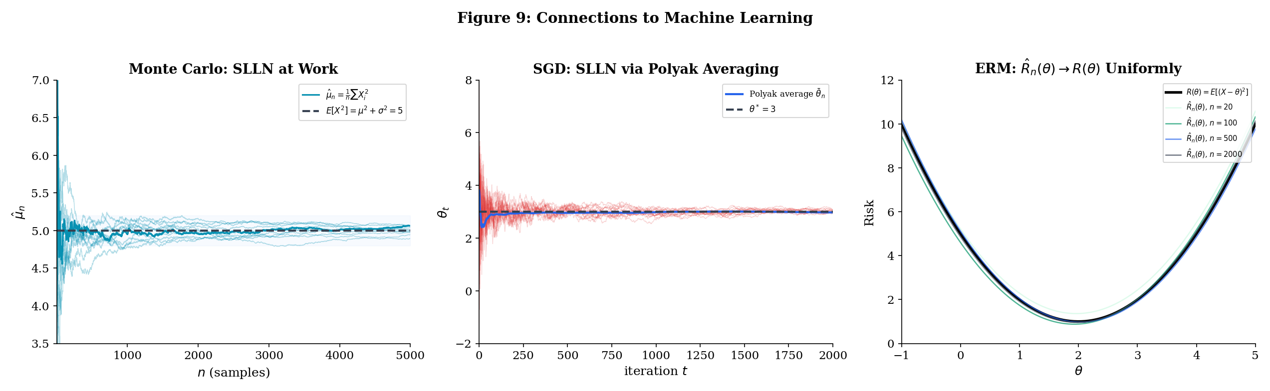
10.9 Connections to Machine Learning
The law of large numbers is not an abstract mathematical curiosity. It is the foundation of empirical machine learning. Every time you compute a statistic from data — a training loss, a validation accuracy, a feature mean for normalization, a gradient estimate — you are implicitly invoking the LLN. The WLLN says your estimate is probably close to the truth. The SLLN says your single run converges to the truth. The Glivenko—Cantelli theorem says the entire empirical distribution converges, not just individual statistics.
This section makes the connections explicit, tracing the LLN through three central pillars of modern ML: Monte Carlo estimation (where the SLLN justifies single-run simulation), stochastic optimization (where the SLLN justifies Polyak averaging), and empirical risk minimization (where the Glivenko—Cantelli theorem justifies training on finite data).
The theme is always the same: we observe a finite sample, compute a statistic (a sample mean, a gradient average, an empirical risk), and trust that it approximates the corresponding population quantity. The LLN is the mathematical warrant for that trust.
It is worth pausing to appreciate the remarkable generality of this foundation. The LLN does not care what the random variables represent — pixel intensities, word embeddings, gradient components, loss values, feature activations. It does not care about the dimension of the underlying space. It does not care about the specific distribution, as long as the mean exists. This universality is what makes the LLN the single most important theorem in applied statistics.
To compute for some function and random variable , draw iid from the distribution of and report:
The SLLN guarantees almost surely — your single simulation run converges to the truth. This is the entire theoretical justification for Monte Carlo estimation.
Concrete example: Suppose and you want to estimate . The true value is . Drawing iid from and computing gives an estimate that converges to 5 almost surely by the SLLN (since ). The CLT will tell us that the error is approximately , giving confidence intervals. And concentration inequalities give non-asymptotic bounds like for bounded transformations — see Hoeffding’s inequality (Theorem 12.3).
The Monte Carlo method extends to high-dimensional integrals where deterministic quadrature fails: if and is large, grid-based methods require evaluations for accuracy (the curse of dimensionality), while Monte Carlo requires only evaluations regardless of — courtesy of the SLLN and CLT.
Notice the role of the SLLN versus the WLLN here. The WLLN would tell you that for each fixed , the probability of your estimate being far from is small. But you are looking at a single run — a single sequence of estimates — and you want this sequence to converge. That is exactly what the SLLN guarantees: with probability 1, your sequence converges to the truth.
The SLLN also extends to MCMC: if the Markov chain is ergodic (irreducible, aperiodic, positive recurrent), then time averages converge to space averages almost surely. This is the ergodic theorem, a generalization of Theorem 10.5 (Kolmogorov/Etemadi SLLN) to dependent sequences — the dependence between successive states of the Markov chain is handled by the ergodic property rather than independence. Topic 26 §26.7 Theorem 5 develops this in the MCMC context. See also formalML: Monte Carlo Methods for applied extensions.
In SGD, we approximate the full gradient with a single-sample gradient . The key convergence result says: with step sizes satisfying the Robbins—Monro conditions ( and ), the iterates converge to a local minimum almost surely.
Polyak averaging replaces the final iterate with the running mean:
This exploits the SLLN: the running mean of the iterates (which fluctuate around the optimum) converges to the optimum almost surely, and the Polyak-averaged estimator achieves the optimal asymptotic variance — it is as efficient as the best possible estimator. The SLLN is what makes this averaging trick valid.
The connection between SGD and the LLN runs deeper than the averaging trick. At each step, the stochastic gradient is a noisy estimate of the true gradient . The noise averages out over time — by the LLN applied to the gradient estimates — and the iterates converge. The Robbins—Monro conditions encode two competing requirements:
- : the step sizes are large enough in total to reach the optimum from any starting point (the algorithm doesn’t stop too early).
- : the step sizes shrink fast enough that the gradient noise averages out (the algorithm doesn’t oscillate forever).
The common choice satisfies both: (harmonic series diverges) and (Basel problem).
See formalML: Stochastic Gradient Descent for the full convergence analysis.
In supervised learning, the empirical risk of a model on data is:
For each fixed , is a sample mean, so the SLLN gives . But ERM selects , and for this to be consistent we need convergence that is uniform over :
This is exactly the type of result that the Glivenko—Cantelli theorem provides for indicator functions , and its generalization to richer function classes (via Vapnik—Chervonenkis theory — proved at Topic 32 §32.4) is what makes ERM work. The function class must be “small enough” — specifically, its VC dimension must be finite — for uniform convergence to hold.
The logical chain from the results in this topic to statistical learning theory is:
- Glivenko—Cantelli (Theorem 10.6): uniform LLN for indicators .
- VC theory (generalization): uniform LLN for function classes with finite VC dimension.
- ERM consistency: the empirical risk minimizer converges to the population risk minimizer.
- PAC learning bounds: with samples, where is the VC dimension.
Each step in the chain uses the previous step as a building block. The Glivenko—Cantelli theorem is step 1 — the simplest case — and everything else follows by generalization.
See formalML: Empirical Risk Minimization and formalML: Generalization Bounds for the full development.
The Glivenko—Cantelli theorem is the simplest case of a uniform law of large numbers. It says that the empirical measure (which assigns mass to each observation) converges to the population measure uniformly over the class of half-lines .
Empirical process theory (Topic 32) generalizes from half-lines to arbitrary function classes , asking: when does ? The answer involves the complexity of — measured by the VC dimension, covering numbers, or metric entropy. The Glivenko—Cantelli class of half-lines has VC dimension 1, which is why the theorem holds without any distributional assumptions.
This is the bridge between the LLN (convergence for a single statistic) and statistical learning theory (uniform convergence over a class of statistics). The function class must be “learnable” (finite VC dimension or, more generally, finite metric entropy) for the uniform LLN to hold, and learnability is equivalent to the uniform LLN. This equivalence — the fundamental theorem of statistical learning — is one of the deepest results in the field.
The Glivenko—Cantelli theorem is the case. This class has VC dimension 1 (any single point can be shattered, but no two points can be). With VC dimension 1, the uniform convergence holds for any distribution — exactly what Theorem 10.6 states.
The extension to higher dimensions is more subtle: in , the class of half-spaces has VC dimension , and the multivariate Glivenko—Cantelli theorem holds with convergence rate — the same rate as in one dimension, independent of . This is remarkable: the empirical CDF converges just as fast in high dimensions as in one dimension, at least for half-spaces. For richer function classes, the rate can degrade with dimension — this is the curse of dimensionality in statistical learning theory.
10.10 Summary
This topic traced the arc from the simplest weak law to the strongest convergence results available for sample means and empirical distributions. Here is the complete progression:
| Result | Assumptions | Conclusion | Proof Tool |
|---|---|---|---|
| Theorem 10.1 (WLLN) | iid, | Chebyshev | |
| Theorem 10.2 (WLLN) | uncorrelated, | Variance of sums | |
| Theorem 10.3 (Khintchine) | iid, | Truncation + DCT | |
| Theorem 10.4 (Kolmogorov) | independent, | Stopping time decomposition | |
| Theorem 10.5 (SLLN) | pairwise iid, | Etemadi (truncation + Kolmogorov + B-C) | |
| Theorem 10.6 (Glivenko—Cantelli) | iid | SLLN for indicators + monotonicity | |
| Theorem 10.7 (Hoeffding) | independent, bounded | (Proof: Topic 12, Theorem 12.3) | |
| Theorem 10.8 (LIL) | iid, | a.s. | (Statement only) |
The logical dependencies form a clear ladder:
- Chebyshev WLLN (Theorem 10.1) is the base case — three lines.
- Uncorrelated WLLN (Theorem 10.2) generalizes by dropping “identically distributed.”
- Khintchine’s WLLN (Theorem 10.3) generalizes by dropping “finite variance,” using truncation.
- Kolmogorov’s maximal inequality (Theorem 10.4) provides the new tool needed to control paths, not just endpoints.
- SLLN (Theorem 10.5) uses Kolmogorov + truncation + Borel—Cantelli to upgrade from “in probability” to “almost surely.”
- Glivenko—Cantelli (Theorem 10.6) uses the SLLN + monotonicity to upgrade from “pointwise” to “uniform.”
At every stage, we relaxed an assumption or strengthened a conclusion. This is how convergence theory works: you start with the simplest result that captures the essential phenomenon, then systematically push the boundaries — either by weakening the hypotheses (making the theorem more broadly applicable) or by strengthening the conclusion (making it more useful). The progression from Theorem 10.1 to Theorem 10.6 exemplifies both directions simultaneously.
The minimal assumption for the LLN is — finite mean. This is both necessary and sufficient (Proposition 10.1). No weaker condition will do. The Cauchy distribution () is the canonical counterexample: its sample mean does not converge, in any mode, to any finite limit. This clean dichotomy — finite mean gives everything, infinite mean gives nothing — is one of the most satisfying results in probability.
For the Glivenko—Cantelli theorem, even the finite-mean assumption is unnecessary: the empirical CDF converges uniformly to the true CDF for every distribution, no matter how heavy the tails. This universality is what makes nonparametric statistics possible — the ECDF is a valid, consistent estimator of any CDF, without distributional assumptions. It is the most assumption-free estimator in all of statistics.
The practical takeaway is reassuring: no matter what your data looks like — Normal, heavy-tailed, multimodal, discrete, continuous, or a bizarre mixture — the empirical CDF faithfully approximates the true CDF, and all statistics derived from the ECDF (quantiles, moments, probabilities of intervals) converge to their population counterparts.
Looking Back: Prerequisites in Action
This topic drew on three specific results from earlier in the curriculum:
- Chebyshev’s inequality (Expectation & Moments, Theorem 12): the proof engine for all three WLLN variants and the starting point for the maximal inequality.
- Borel—Cantelli lemma (Modes of Convergence): used in the SLLN proof (truncation error vanishes a.s.) and the Glivenko—Cantelli proof (finite intersection of probability-1 sets). The first Borel—Cantelli requires only ; the second (used in Proposition 10.1) requires independence.
- Dominated convergence theorem ( formalCalculus: The Riemann Integral & FTC ): the key tool in every truncation argument — it justifies and . The DCT appeared in three steps of the Khintchine proof and two steps of the Etemadi proof.
The four modes of convergence from Topic 9 provided the conceptual framework: the WLLN is a convergence-in-probability statement, the SLLN is an almost-sure convergence statement, and the hierarchy theorem (a.s. implies in probability, Topic 9 Theorem 9.5) means the SLLN is strictly stronger. The Glivenko—Cantelli theorem adds a new dimension: not just convergence of a single statistic, but uniform convergence of an entire function.
What Comes Next
The law of large numbers says . Two natural follow-up questions remain:
-
What is the shape of the fluctuations? The Central Limit Theorem answers this: . The deviations of from , when rescaled by , are approximately Normal — regardless of the underlying distribution of , as long as the variance is finite. This universality is what makes confidence intervals, hypothesis tests, and p-values work. The CLT says the LLN’s fluctuations are Gaussian in shape — and from that shape, all of classical statistics flows.
The CLT is the distributional complement to the LLN’s qualitative statement. The LLN says ; the CLT says how deviates from at scale .
-
How fast does the convergence happen? Large Deviations & Tail Bounds answers this with exponential-rate guarantees. Hoeffding’s inequality (previewed in Theorem 10.7, proved in Topic 12 as Theorem 12.3) is the simplest such bound; Bernstein’s inequality gives tighter results when the variance is small; sub-Gaussian and sub-exponential tail bounds handle the most common distributional families. These are the finite-sample tools that power statistical learning theory: PAC bounds, uniform convergence rates, and sample complexity calculations — all developed in Large Deviations & Tail Bounds.
These concentration inequalities are the quantitative complement to the LLN’s qualitative statement. The LLN says ; the concentration inequalities say exactly how many samples you need for with probability at least .
Together, the LLN (convergence), the CLT (the shape), and concentration inequalities (the rate) form the three pillars of asymptotic statistics. Everything in statistical inference — point estimation, confidence intervals, hypothesis testing, Bayesian asymptotics — rests on one or more of these pillars. The LLN says “your estimator works.” The CLT says “here is how to quantify your uncertainty.” Concentration inequalities say “here is exactly how many samples you need.”
With the LLN now proved, we have the first of these three pillars firmly in place. The sample mean converges to the truth — weakly under finite variance, strongly under finite mean, uniformly for the empirical CDF. The next two topics will complete the trinity.
The reader who has followed from Topic 1 (Sample Spaces) through Topic 10 has now traversed the full journey from “what is a random event?” to “sample means converge almost surely to population means.” This is the first genuinely asymptotic result in the curriculum — a statement about what happens as — and it opens the door to all of statistical inference. Point estimation relies on the SLLN for consistency. Confidence intervals rely on the CLT (which refines the LLN). Hypothesis testing relies on the asymptotic distribution of test statistics (which follows from the CLT). Bayesian consistency (the posterior concentrating around the true parameter) relies on the SLLN for the log-likelihood. Every branch of inference grows from this root.
References
- Durrett, R. (2019). Probability: Theory and Examples (5th ed.). Cambridge University Press.
- Billingsley, P. (2012). Probability and Measure (Anniversary ed.). Wiley.
- Casella, G. & Berger, R. L. (2002). Statistical Inference (2nd ed.). Duxbury.
- Etemadi, N. (1981). An elementary proof of the strong law of large numbers. Zeitschrift für Wahrscheinlichkeitstheorie und verwandte Gebiete, 55, 119–122.
- Wasserman, L. (2004). All of Statistics. Springer.
- Bishop, C. M. (2006). Pattern Recognition and Machine Learning. Springer.