Exponential Families
Nine distributions, one canonical form — the unifying framework that makes sufficient statistics, MLE, conjugate priors, and GLMs tractable.
7.1 The Exponential Family (Why Unify?)
Topic 5 — Discrete Distributions cataloged seven discrete PMFs and flagged five as exponential family members. Topic 6 — Continuous Distributions cataloged eight continuous PDFs and flagged four more. In both cases, the exponential family membership was noted in passing — a remark here, a flag there — without explaining what that membership means or why it matters.
This topic answers that question. Nine of the sixteen distributions from Topics 5-6 — Bernoulli, Binomial, Geometric, Negative Binomial, Poisson, Normal, Exponential, Gamma, and Beta — share a single algebraic form:
This is not a coincidence, and it is not merely a notational convenience. The factorization above — in which the data and the parameter interact only through the inner product — is the structural reason behind four of the most important results in parametric statistics:
- Sufficient statistics are finite-dimensional. The function captures everything the data has to say about . No matter how large the sample, a fixed-dimensional summary suffices.
- MLE reduces to moment matching. The maximum likelihood estimate satisfies , where is the sample mean of the sufficient statistics. One equation, universal across all nine distributions.
- Conjugate priors exist. For every exponential family likelihood, there is a natural conjugate prior that yields a posterior in the same family — with hyperparameters updated by a clean additive rule.
- Generalized linear models are tractable. The GLM framework — logistic regression, Poisson regression, Gamma regression — requires an exponential family response distribution. The canonical link function comes directly from .
The distributions that are not exponential family members — Hypergeometric, Discrete Uniform, Continuous Uniform, Student’s , and — fail for specific structural reasons that we will make precise in Section 7.4. The Chi-squared distribution, by contrast, is a special case of the Gamma and therefore belongs to the exponential family; we do not count it separately among the nine because its degrees-of-freedom parameter is typically treated as a fixed integer, not an estimated parameter.
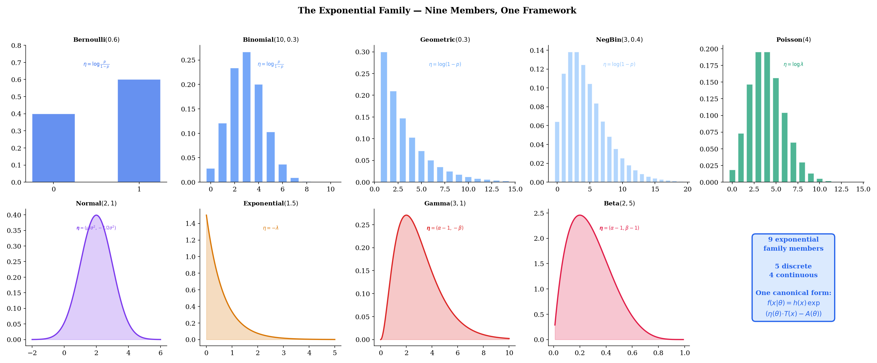
The interactive explorer below lets you select any of the nine members, adjust parameters, and see the canonical form decomposition live — with the four components , , , and color-coded in the formula.
7.2 The Canonical Form
Before we can unify nine distributions, we need a precise definition of the form they share. We start with the one-parameter case to build intuition, then generalize.
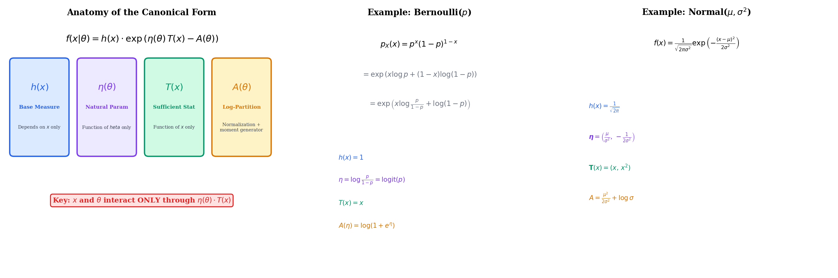
A family of distributions indexed by a scalar parameter is a one-parameter exponential family if the PMF or PDF can be written as
where:
- is a base measure that depends only on the data, not on
- is the natural parameter (also called the canonical parameter), a function of alone
- is the sufficient statistic, a function of the data alone
- is the log-partition function (also called the cumulant function), which ensures the density integrates to 1
The key structural feature is that and interact only through the product . Everything else separates cleanly: absorbs the data-only terms, and absorbs the parameter-only normalization.
When — that is, when the natural parameter is the parameter — we say the family is in natural or canonical parameterization. This is always achievable by reparameterizing from to .
The generalization to multiple parameters is immediate.
A family of distributions indexed by a parameter vector is a -parameter exponential family if the PMF or PDF can be written as
where is a vector of natural parameters, is a vector of sufficient statistics, and the dot product replaces the scalar product. The log-partition function normalizes the distribution.
The dimension of the exponential family is — the number of natural parameters. The Bernoulli, Geometric, Poisson, and Exponential are one-dimensional (). The Normal, Gamma, and Beta are two-dimensional (). The Binomial and Negative Binomial are one-dimensional when (resp. ) is fixed.
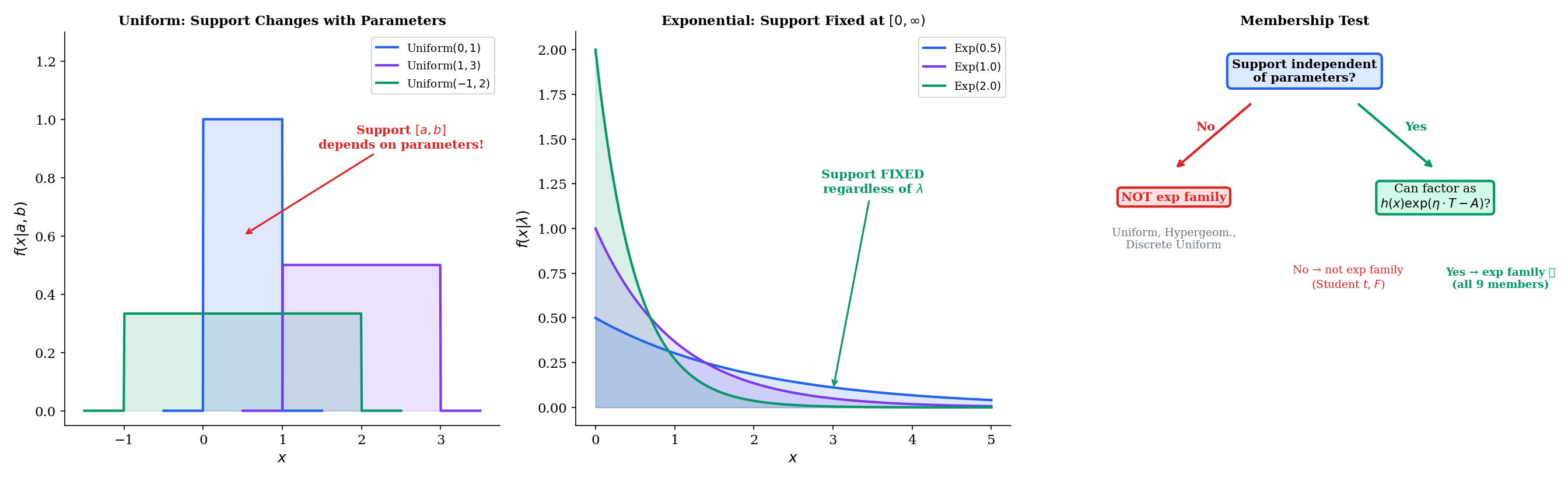
A critical requirement — often stated implicitly — is that the support of must be independent of . The set of values where must be the same for all .
Why? Because is the only factor that can restrict the support (by being zero), and does not depend on . If the support depends on , we would need an indicator function that cannot be absorbed into the structure.
This is exactly why the Uniform distribution fails to be an exponential family member, as we will see in Section 7.4.
7.3 Converting Distributions to Canonical Form
We now convert all nine exponential family members to canonical form. The method is the same in every case: start with the known PMF or PDF from Discrete Distributions or Continuous Distributions, take the logarithm, separate the terms that involve only , only , and both and , then read off , , , and .
These conversions are compressed — the full PMF/PDF derivations live in Topics 5-6, so we start from the final expressions and focus on the algebraic rearrangement.
7.3.1 Bernoulli
The Bernoulli PMF is for . Taking the logarithm:
Reading off the components:
- (the log-odds, also called the logit)
- (the softplus function)
The natural parameter ranges over all of : as , ; as , . The inverse map is , the logistic function — and this is exactly why logistic regression uses the logit link.
7.3.2 Binomial (fixed )
The Binomial PMF is for , with fixed. Taking the logarithm:
Reading off:
- (same logit as Bernoulli)
The Binomial with fixed is a one-parameter exponential family in . When both and are unknown, the family is no longer exponential in the standard sense because enters through , which couples data and parameters outside the structure.
7.3.3 Geometric
The Geometric PMF is for (counting the trial on which the first success occurs). Taking the logarithm:
Reading off:
Since , we have , so . The natural parameter space is .
7.3.4 Negative Binomial (fixed )
The Negative Binomial PMF is for , with fixed. Taking the logarithm:
Reading off:
The natural parameter space is , identical to the Geometric. This makes sense: the Geometric is the Negative Binomial with , and setting in recovers the Geometric log-partition function exactly when .
7.3.5 Poisson
The Poisson PMF is for . Taking the logarithm:
Reading off:
The natural parameter ranges over all of (since ). The log-partition function is the exponential function itself — making the Poisson the cleanest example for studying and its derivatives.
7.3.6 Normal
The Normal PDF is for . This is a two-parameter family. Expanding the exponent:
So the full log-density is:
Reading off:
- , so and
The natural parameter space is , . When is known, the Normal reduces to a one-parameter exponential family with natural parameter , sufficient statistic , and log-partition function .
7.3.7 Exponential
The Exponential PDF is for . Taking the logarithm:
Reading off:
- for
The natural parameter (since ). Note the sign: the natural parameter is the negative of the rate. This is a one-parameter exponential family with natural parameter space .
7.3.8 Gamma
The Gamma PDF is for . Taking the logarithm:
This is a two-parameter family. Reading off:
- for
- , so and
The natural parameter space is , . Setting (i.e., ) and keeping only the second component recovers the Exponential canonical form: , , . The Gamma genuinely subsumes the Exponential as a special case, and the canonical forms are consistent.
7.3.9 Beta
The Beta PDF is for . Taking the logarithm:
Reading off:
- for
- , so and
The natural parameter space is , . The sufficient statistics and are the log-data and the log-complement — both of which appear naturally in the Beta-Bernoulli conjugate updating that we will derive in Section 7.7.
The converter below lets you step through the algebraic transformation for each distribution, with color-coded components matching the canonical form.
Interactive: Canonical Form Converter
7.4 Why Some Distributions Are NOT Exponential Families
Not every distribution fits the canonical form. Of the sixteen distributions cataloged in Topics 5-6, seven are excluded. Understanding why they fail sharpens our understanding of what the exponential family structure actually requires.
The Student’s PDF is proportional to , and the PDF involves a similar power-of-a-polynomial structure. In both cases, the parameter (, or ) appears as an exponent on a function of . There is no way to factor the log-density into a sum plus separate functions of and alone.
Concretely, for the distribution:
The term cannot be written as because appears both as a multiplicative factor () and inside the argument of the logarithm (). This double entanglement of data and parameter prevents the factorization.
The same issue affects the distribution. Both are derived from the Normal and Chi-squared via ratios and transformations that destroy the exponential family structure.
The Continuous Uniform has PDF
where is the indicator function that equals 1 when and 0 otherwise. The support of is the interval , which depends on the parameters and .
We can try to force this into exponential family form by taking the log:
The indicator equals 0 when and otherwise. This indicator depends on both and , but it cannot be written as — it is a hard constraint, not a smooth inner product.
The Discrete Uniform fails for exactly the same reason: its support depends on the parameters. The Hypergeometric fails similarly: its support depends on .
This is the content of Remark 7.1: the support of an exponential family density must be independent of the parameter. Parameter-dependent support is the most common reason a distribution fails the exponential family test.
7.5 The Log-Partition Function
The log-partition function is the most important single object in exponential family theory. Its name comes from statistical mechanics, where is the partition function — the normalizing constant that ensures probabilities sum (or integrate) to 1. But does far more than normalize. Its derivatives generate the moments of the sufficient statistic.
Let be a one-parameter exponential family in natural parameterization. Then:
In words: the first derivative of the log-partition function gives the expected value of the sufficient statistic, and the second derivative gives its variance.
Proof [show]
Part 1. The density integrates to 1 for all in the natural parameter space:
Multiply both sides by :
Differentiate both sides with respect to . On the left, we differentiate under the integral sign (justified by the smoothness of exponential families on the interior of the natural parameter space — see Barndorff-Nielsen, Ch. 8):
Divide both sides by :
The left side is . Therefore .
Part 2. Differentiate the normalization identity a second time. Starting from
we differentiate both sides with respect to again. On the left:
On the right, by the product rule:
Divide both sides by :
The left side is . Since , we have:
Rearranging: .
Let us verify this on the cleanest example. For the Poisson, , so and . We know and for the Poisson — both confirmed by the log-partition derivatives. For the Bernoulli, , so and , matching and .
Since (variance is nonnegative), the log-partition function is convex. Moreover, whenever is not degenerate (i.e., takes more than one value with positive probability), so is strictly convex for all standard exponential families.
This has three major consequences:
-
The log-likelihood is concave. For a sample , the log-likelihood in natural parameterization is . Since is convex, is concave, and is a linear function plus a concave function — hence concave. This guarantees that any local maximum of the log-likelihood is the global maximum.
-
The MLE is unique (when it exists). A strictly concave function has at most one maximum. Combined with existence conditions (the observed sufficient statistic lies in the interior of the convex hull of possible sufficient statistics), this gives both existence and uniqueness of the MLE.
-
The mean-to-natural parameter map is invertible. The function is strictly increasing (since ), so it has an inverse . This invertibility is what makes the dual parameterization — sometimes called the mean parameterization — well-defined.
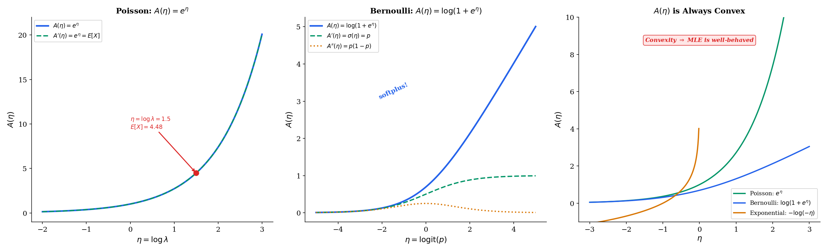
The explorer below lets you drag a point along the axis and watch , , and update in real time. The tangent line at each point has slope .
A(η) is convex → log-likelihood is concave → MLE exists and is unique
7.6 Sufficient Statistics from Exponential Families
The canonical form immediately reveals the sufficient statistic — but why is sufficient? The answer comes from the Fisher-Neyman factorization theorem, which states that is sufficient for if and only if the density factors as a function of and times a function of alone.
In any exponential family , the statistic is sufficient for .
For an i.i.d. sample from this family, the sum is sufficient for .
Proof [show]
The Fisher-Neyman factorization theorem (which Sufficient Statistics develops in full generality) states that is sufficient for if and only if the joint density factors as
where depends on only through , and depends only on .
For an exponential family, the density is already in this form:
The first factor depends on only through (since the data enters only via the inner product ). The second factor depends only on , not on . The factorization is immediate.
For an i.i.d. sample, the joint density is . The same factorization holds with playing the role of the sufficient statistic and playing the role of the data-only factor.
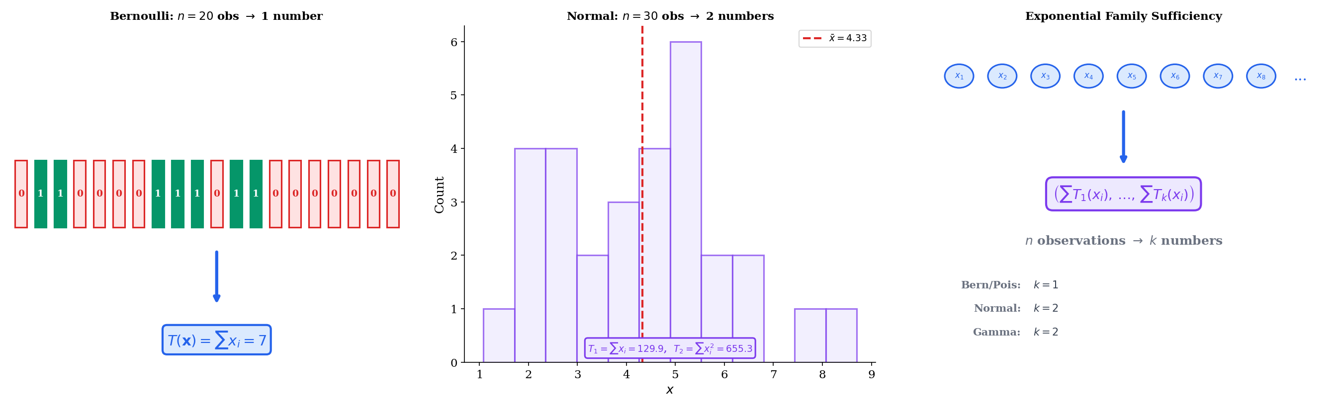
The power of this result is dimensional reduction. No matter how large the sample, a fixed-dimensional summary suffices:
- Bernoulli: , so — the number of successes. One number summarizes binary observations.
- Normal (known ): , so , or equivalently . One number summarizes continuous observations.
- Normal (unknown and ): , so the sufficient statistics are and . Two numbers summarize the entire sample.
- Poisson: , so — the total count. One number.
This is not a feature of specific distributions — it is a structural consequence of the exponential family form. Sufficient Statistics develops the full theory, including the Rao-Blackwell theorem (sufficient statistics yield optimal estimators), completeness (no redundancy in the sufficient statistic), and the Pitman-Koopman-Darmois converse: under regularity, exponential families are the ONLY families admitting fixed-dimensional sufficient statistics as n grows.
7.7 Conjugate Priors from Exponential Families
One of the most elegant consequences of the exponential family structure is the existence of conjugate priors. A conjugate prior for a likelihood is a prior distribution such that the posterior belongs to the same family as the prior — just with updated parameters. This makes Bayesian updating algebraically tractable: multiply the prior by the likelihood, and read off the new parameters without computing a normalizing integral.
The remarkable fact is that every exponential family has a natural conjugate prior. The general form is a direct consequence of the canonical representation.
Let be a one-parameter exponential family in natural parameterization. The conjugate prior for has the form
where and are hyperparameters.
Given an i.i.d. sample , the posterior is in the same family with updated hyperparameters:
where is the sample mean of the sufficient statistics.
Proof [show]
The likelihood for an i.i.d. sample from an exponential family is:
The product does not depend on and will be absorbed into the proportionality constant. Writing :
Multiply by the conjugate prior :
This is the same functional form as the prior, with replaced by and replaced by . The posterior is therefore in the conjugate family.
The hyperparameter acts as a pseudo-sample size: it measures how much weight the prior carries relative to the data. After observing real data points, the effective sample size increases from to . The hyperparameter acts as a pseudo-sufficient-statistic sum: it represents the “data” implied by the prior, and it is updated additively by the observed sufficient statistic sum .
The theorem above is the general result. Let us see it in action for three specific conjugate pairs.
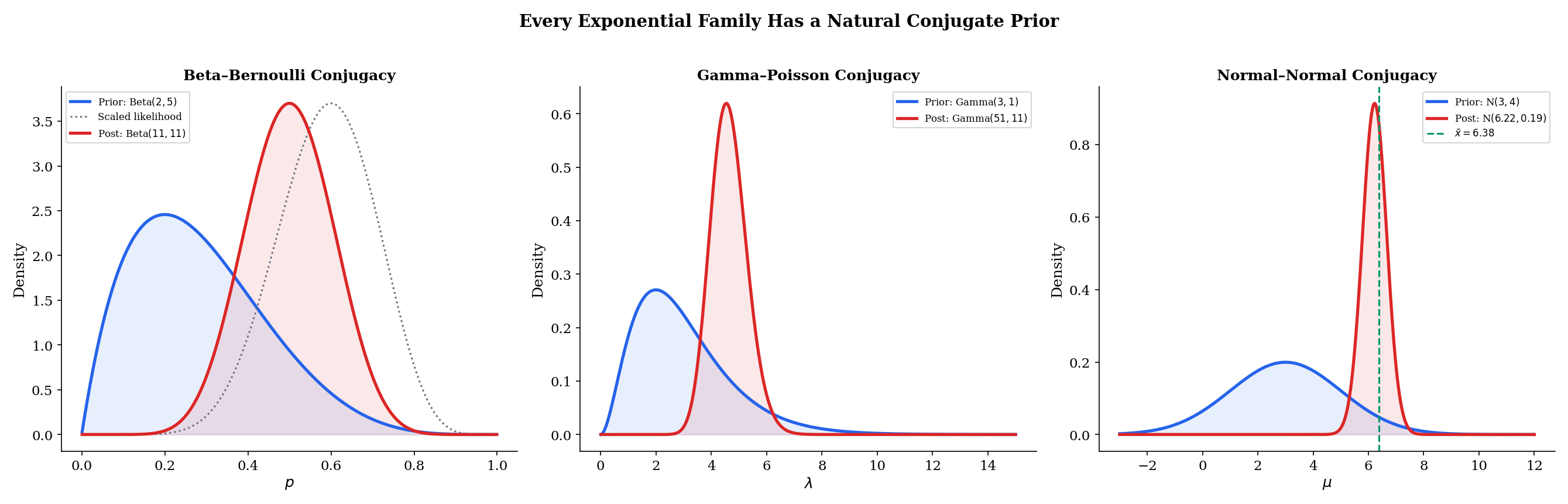
For the Bernoulli with natural parameter and log-partition , the conjugate prior is
Given Bernoulli observations with successes (so ), the posterior is:
In the general framework: (pseudo-successes minus 1), (pseudo-sample-size minus 2), and the update rule gives , . The Beta parameterization absorbs the offsets.
The posterior mean is — a weighted average of the prior mean and the sample proportion , with weights proportional to the pseudo-sample size and the real sample size.
For the Poisson with natural parameter and log-partition , the conjugate prior for is
Given Poisson observations with total count , the posterior is:
The update rule is clean: accumulates the total count, accumulates the number of observations. The posterior mean is — a weighted average of the prior mean and the sample mean .
For the Normal with known variance , the natural parameter is and the log-partition is . The conjugate prior for is
Given Normal observations with sample mean , the posterior is:
where the posterior variance and mean are given by the precision-weighted average:
The posterior precision (inverse variance) is the sum of the prior precision and the data precision. The posterior mean is the precision-weighted average of the prior mean and the sample mean. As , the data precision dominates and — the posterior concentrates on the MLE, regardless of the prior. This is a concrete instance of posterior consistency.
The explorer below lets you experiment with all three conjugate pairs. Adjust the prior hyperparameters, add data, and watch the posterior concentrate.
7.8 Maximum Likelihood in Exponential Families
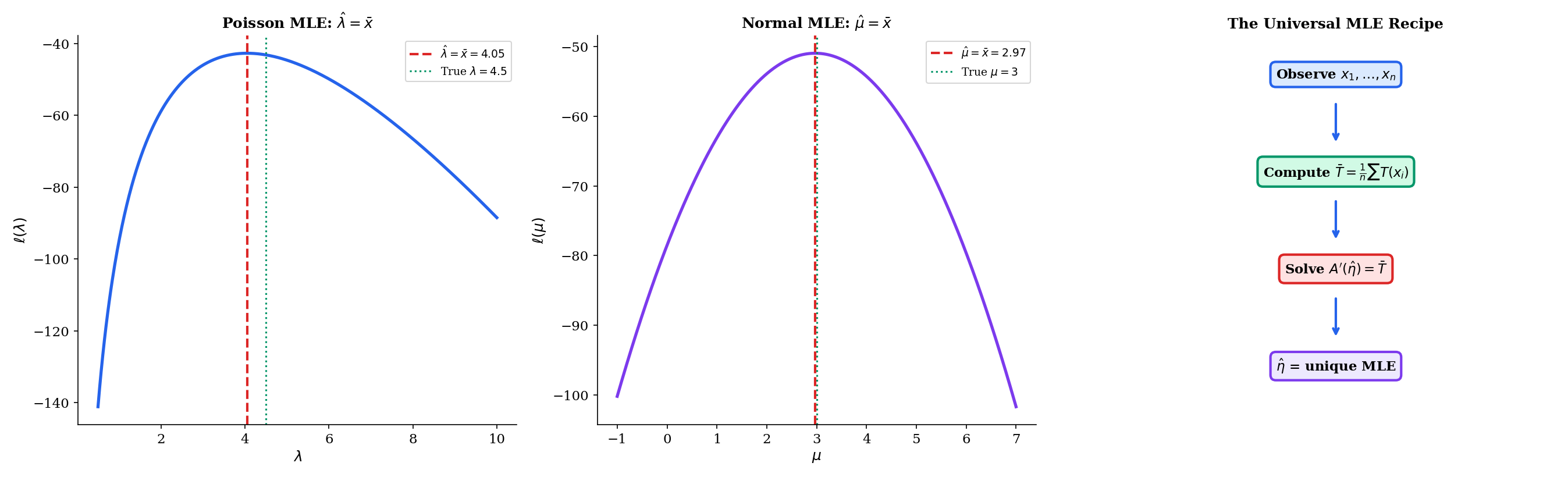
The log-partition function’s properties give us a universal recipe for maximum likelihood estimation that applies to all nine exponential family members simultaneously.
Let be an i.i.d. sample from a one-parameter exponential family . The maximum likelihood estimator satisfies
where is the sample mean of the sufficient statistics. When lies in the interior of the range of , this equation has a unique solution.
Proof [show]
The log-likelihood for an i.i.d. sample is:
The first sum does not depend on . Writing :
Differentiate with respect to and set to zero:
This is the score equation. It says: find the parameter value such that the model’s expected sufficient statistic equals the observed sufficient statistic . This is moment matching — the MLE equates the theoretical and empirical moments of the sufficient statistic.
Existence. By Theorem 7.1, . The range of is an open interval (by the strict convexity of and the intermediate value theorem). If lies in this interval, the equation has a solution.
Uniqueness. Since , the function is strictly increasing. A strictly increasing function can hit each value at most once, so the solution is unique.
Global maximum. The second derivative of the log-likelihood is , so the log-likelihood is strictly concave. Any critical point is the unique global maximum.
The universal recipe specializes to every distribution’s MLE formula. Let us verify the four most important cases.
For the Poisson: , , , so . The MLE equation becomes
The Poisson MLE is the sample mean — the most natural estimator one could imagine, and now we see it is a consequence of the exponential family structure. The existence condition is , which holds whenever at least one observation is nonzero.
For the Bernoulli: , , , so . The MLE equation becomes
where is the number of successes. The sample proportion is the MLE for the Bernoulli probability — again, a universally known result that falls out automatically from .
For the Exponential: , , , so . The MLE equation becomes
The MLE for the Exponential rate is the reciprocal of the sample mean. The existence condition is , which holds for any sample from a continuous positive distribution.
For the Normal with known : , , , so . The MLE equation becomes
The sample mean is the MLE for the Normal mean — the single most foundational result in point estimation, and it requires exactly one line once we have the exponential family machinery. Maximum Likelihood Estimation develops the general theory, including asymptotic properties and the multiparameter case.
7.9 Connection to Generalized Linear Models
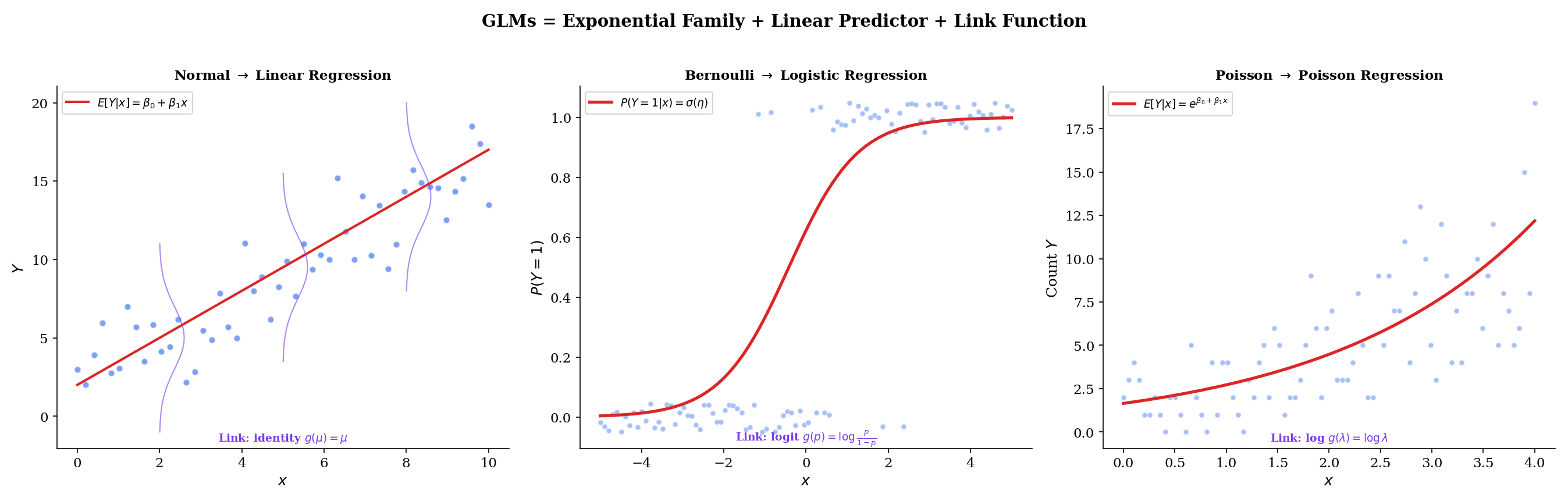
The exponential family is not just a theoretical convenience — it is the structural foundation of generalized linear models (GLMs), arguably the most widely used class of statistical models in applied science and industry. Every GLM has three components: a random component (the response distribution), a systematic component (the linear predictor ), and a link function connecting them. The exponential family determines the first and third components.
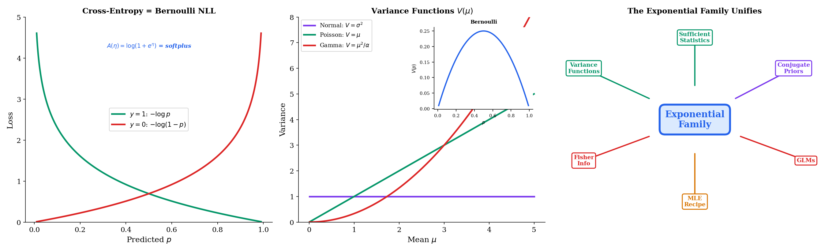
For any exponential family member, the variance function expresses the variance of the response as a function of its mean:
The variance function characterizes the mean-variance relationship and determines the behavior of the GLM. For the Normal, (constant variance). For the Poisson, (variance equals the mean). For the Bernoulli, (variance is maximized at ). For the Gamma, (variance grows quadratically with the mean).
These variance functions dictate when each GLM is appropriate: Poisson regression for count data where variance scales with the mean, Gamma regression for positive continuous data where variance scales with the square of the mean, logistic regression for binary data with the bell-shaped variance curve.
The canonical link function for a GLM is , which maps the mean response directly to the natural parameter . When we use the canonical link, the linear predictor equals the natural parameter: .
| Distribution | Canonical link | Link name | GLM |
|---|---|---|---|
| Normal | Identity | Linear regression | |
| Bernoulli | Logit | Logistic regression | |
| Poisson | Log | Poisson regression | |
| Gamma | Inverse | Gamma regression |
Linear regression is the Normal GLM with identity link: . The mean is the linear predictor.
Logistic regression is the Bernoulli GLM with logit link: . The log-odds is the linear predictor.
Poisson regression is the Poisson GLM with log link: . The log-mean is the linear predictor.
In each case, the canonical link emerges directly from the exponential family structure — it is the function that maps from the mean parameterization to the natural parameterization. Generalized Linear Models develops the full theory, including non-canonical links, iteratively reweighted least squares, and deviance analysis.
The variance function determines the weight structure of the GLM. In weighted least squares terms, the weight for observation is inversely proportional to :
| Distribution | Behavior | Implication | |
|---|---|---|---|
| Normal | (constant) | Constant variance | OLS is optimal |
| Poisson | Variance = mean | Overdispersion is common | |
| Bernoulli | Variance peaks at | Observations near or are more informative | |
| Gamma | Variance mean | Coefficient of variation is constant |
When the variance function does not match the data’s actual mean-variance relationship, we get misspecification. Poisson regression with applied to overdispersed count data (where the true variance is for some ) produces correct point estimates but anticonservative standard errors. The Negative Binomial, with , is the standard remedy.
7.10 Connections to ML
The exponential family is not an abstract mathematical curiosity — it is the structural backbone of modern machine learning. Cross-entropy loss, Fisher information, natural gradients, and variational inference all trace back to the canonical form.
The binary cross-entropy loss used in every classification neural network is
This is exactly the negative log-likelihood of a single Bernoulli observation with parameter :
In natural parameterization, with , the loss becomes , which is the exponential family negative log-likelihood up to a constant.
When a neural network’s final layer applies a sigmoid activation and is trained with binary cross-entropy, it is performing maximum likelihood estimation for a Bernoulli exponential family model with natural parameter . This is logistic regression. The entire deep learning classification pipeline — softmax output, cross-entropy loss, gradient descent — is exponential family MLE in disguise.
The Fisher information for a one-parameter exponential family in natural parameterization is
This is a consequence of Theorem 7.1: the Fisher information equals the second derivative of the log-partition function, which equals the variance of the sufficient statistic. For an i.i.d. sample of size , the Fisher information is .
The Fisher information defines a Riemannian metric on the parameter space. The “distance” between two parameter values and is not the Euclidean distance but the geodesic distance measured by . This is the starting point of formalML: , which studies the differential geometry of statistical models.
Natural gradient descent replaces the standard gradient update with the natural gradient . This rescales the gradient by the inverse Fisher information, making the update invariant to reparameterization. For exponential families, the natural gradient has a clean form because is readily computable. formalML: exploits this: when the variational distribution is an exponential family, the natural gradient of the ELBO has a closed-form update.
Summary
The exponential family is the single most important structural concept in parametric statistics. Nine distributions, one canonical form, and four major consequences: sufficient statistics, conjugate priors, a universal MLE recipe, and the GLM framework.
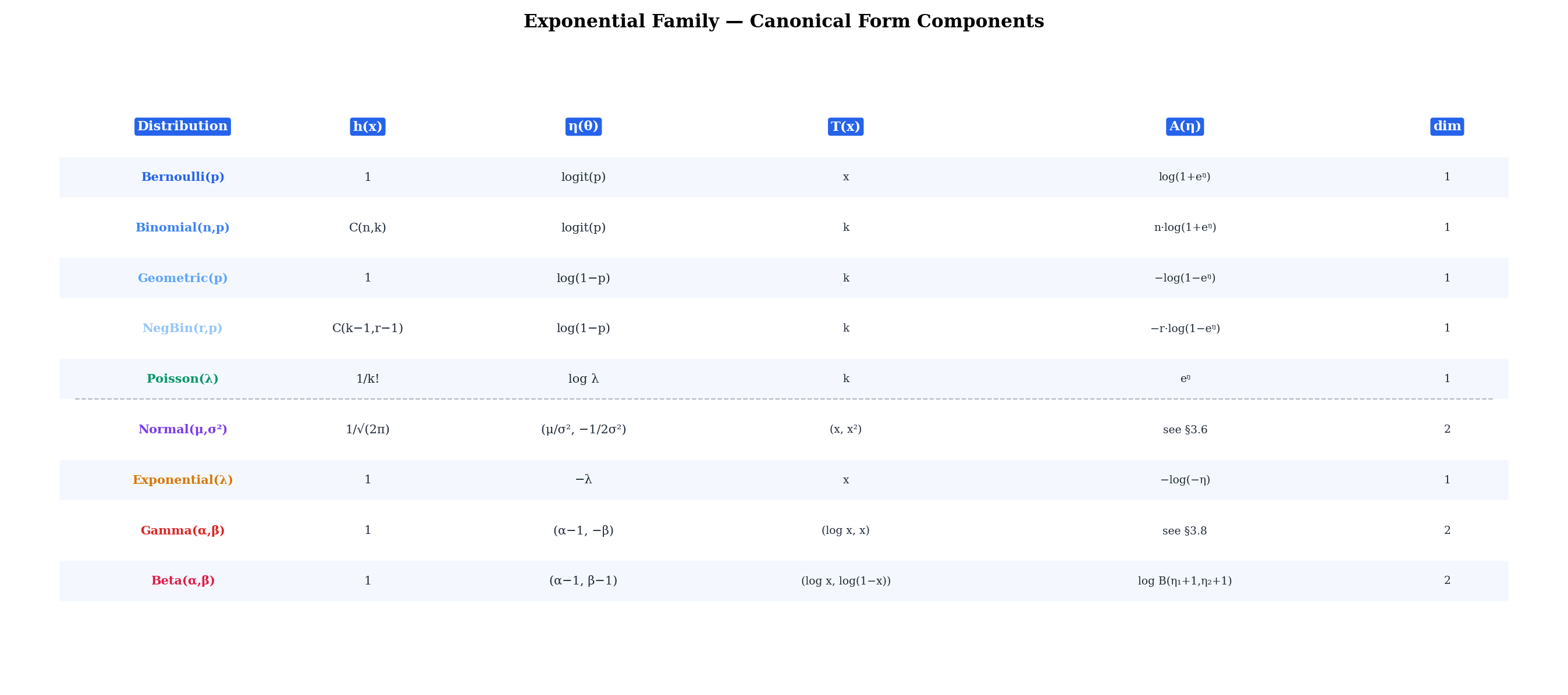
| Distribution | Dim | ||||
|---|---|---|---|---|---|
| Bernoulli | 1 | ||||
| Binomial | 1 | ||||
| Geometric | 1 | ||||
| NegBin | 1 | ||||
| Poisson | 1 | ||||
| Normal | 2 | ||||
| Exponential | 1 | ||||
| Gamma | 2 | ||||
| Beta | 2 |
The log-partition function is the central object. Its first derivative gives , its second derivative gives and the Fisher information , and its convexity guarantees the concavity of the log-likelihood.
The canonical form determines the MLE. The universal recipe — match the model’s expected sufficient statistic to the sample’s observed sufficient statistic — yields every distribution’s MLE formula in one line.
The canonical form determines conjugate priors. Every exponential family has a natural conjugate prior with the update rule , , specializing to Beta-Bernoulli, Gamma-Poisson, and Normal-Normal.
The canonical form determines GLMs. The canonical link function connects the linear predictor to the natural parameter. Logistic regression, Poisson regression, and Gamma regression are all instances.
What comes next. This topic established the unifying framework. The downstream topics build on it:
- Sufficient Statistics develops the full theory of data reduction, including the Rao-Blackwell theorem, completeness, Lehmann-Scheffé UMVUE, Basu’s independence theorem, and the Pitman-Koopman-Darmois converse, building directly on the sufficient statistic identified here
- Maximum Likelihood Estimation develops the asymptotic theory of MLE — consistency, asymptotic normality, efficiency — using the exponential family as the primary example class
- Bayesian Foundations (Topic 25) develops the full Bayesian framework. The §7.7 conjugate prior theorem becomes Topic 25’s Thm 2, lifted into the Bayesian inferential framework with credible intervals, posterior predictive, and Bernstein–von Mises asymptotics
- Generalized Linear Models develops the complete GLM framework — estimation via IRLS, deviance, model diagnostics — requiring the exponential family response distribution established here
For the connections to machine learning at scale, see formalML: (Fisher information as Riemannian metric, natural gradient descent), formalML: (logistic, Poisson, and Gamma regression), and formalML: (exponential family variational distributions and natural gradient VI).
References
- Casella, G. & Berger, R. L. (2002). Statistical Inference (2nd ed.). Duxbury.
- Bickel, P. J. & Doksum, K. A. (2015). Mathematical Statistics: Basic Ideas and Selected Topics (2nd ed.). Chapman and Hall/CRC.
- McCullagh, P. & Nelder, J. A. (1989). Generalized Linear Models (2nd ed.). Chapman & Hall/CRC.
- Bishop, C. M. (2006). Pattern Recognition and Machine Learning. Springer.
- Barndorff-Nielsen, O. E. (2014). Information and Exponential Families in Statistical Theory (2nd ed.). Wiley.
- Efron, B. (2022). Exponential Families in Theory and Practice. Cambridge University Press.