Modes of Convergence
Almost sure, in probability, in distribution, in Lp — the hierarchy and when each matters.
9.1 Why Convergence Needs Four Definitions
Topics 1 through 8 built the vocabulary of probability: sample spaces gave us the stage, random variables gave us the actors, distributions told us how the actors behave, and moments — expectation, variance, the MGF — gave us numerical summaries of that behavior. But vocabulary alone doesn’t make a language. We need grammar — rules for combining simple objects into complex ones and understanding what happens when we take limits.
This topic starts that grammar. The central question is deceptively simple: if is a sequence of random variables, what does it mean to say that converges to some random variable ?
For deterministic sequences, there is exactly one answer. A sequence converges to if for every there exists such that for all . The - definition from calculus handles everything.
For random variables, the situation is fundamentally different. A random variable is a function from the sample space to the real numbers, so asking whether converges to is asking whether a sequence of functions converges. And functions can converge in many different ways.
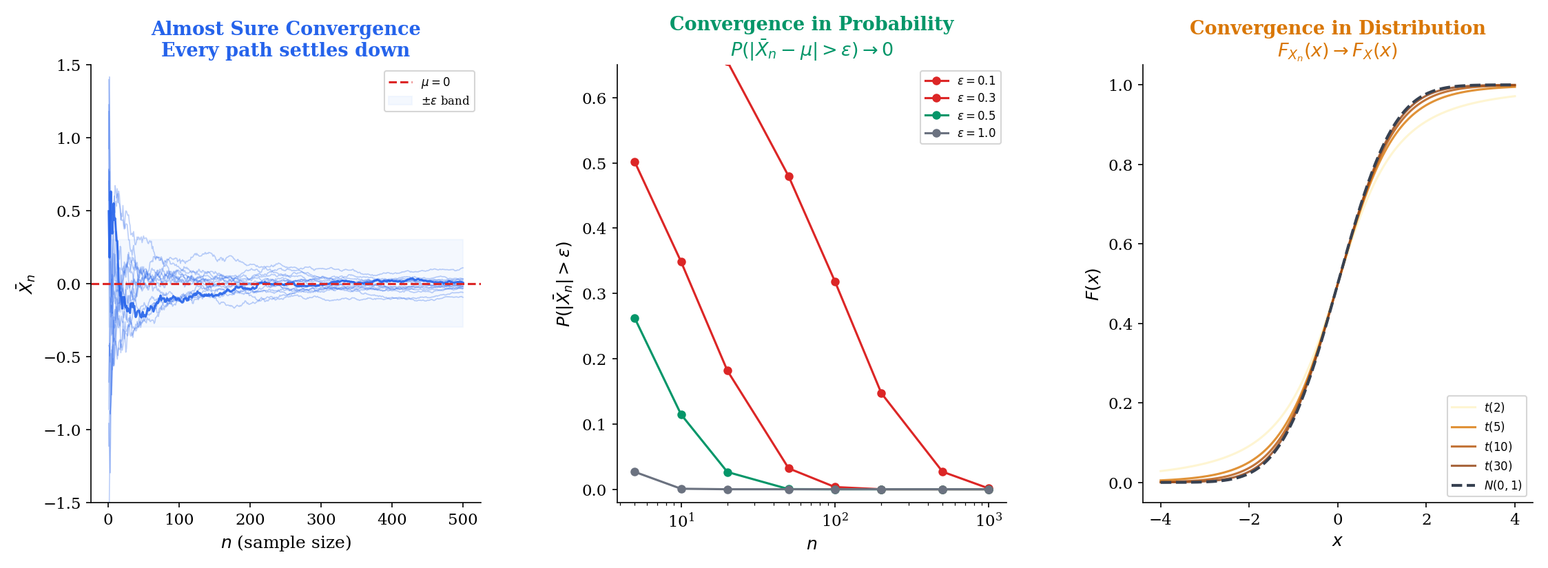
Consider the most important sequence in statistics: the sample mean , where the are iid with mean . We want to say . But what exactly does this mean?
- Does every single realization of the sample mean eventually settle near ? (That’s a strong demand — it requires every sample path to converge.)
- Or do we only need that the probability of being far from goes to zero? (That’s weaker — some paths might misbehave, as long as the misbehaving paths become rare.)
- Or do we only need that the distribution of concentrates around ? (That’s weaker still — we’re just comparing CDFs.)
These three questions lead to genuinely different notions of convergence, and a fourth emerges when we bring moment conditions into the picture. Here are the four modes, in preview:
| Mode | Notation | Intuition |
|---|---|---|
| Almost sure | Every sample path converges | |
| In | The -th moment of the gap vanishes | |
| In probability | Deviations become rare | |
| In distribution | CDFs converge at continuity points |
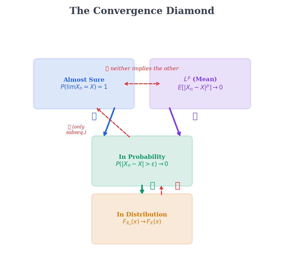
These four modes form a strict hierarchy — a diamond, not a line — with almost sure and at the top, convergence in probability in the middle, and convergence in distribution at the bottom. The arrows point downward: stronger modes imply weaker ones, but not the reverse. Section 9.6 will make this precise, and Section 9.7 will show, with explicit counterexamples, exactly why the arrows don’t reverse.
The tools that launch convergence theory are all from Topic 4 — Expectation, Variance & Moments: Markov’s inequality (Theorem 11), Chebyshev’s inequality (Theorem 12), Jensen’s inequality (Theorem 13), and MGF uniqueness (Theorem 17). Chebyshev gives us convergence in probability (Section 9.2). MGF convergence gives us convergence in distribution (Section 9.5). Jensen and Markov bridge between and probability modes (Section 9.6). If any of these results feel unfamiliar, revisit Topic 4, Sections 5 and 7, before proceeding.
We start with convergence in probability — not because it’s the strongest mode, but because it follows directly from a tool the reader already knows: Chebyshev’s inequality.
9.2 Convergence in Probability
Chebyshev’s inequality (Topic 4, Theorem 12) tells us that . If the variance of a sequence shrinks to zero, then the probability of large deviations also goes to zero. This is the intuition behind convergence in probability.
A sequence of random variables converges in probability to a random variable if for every ,
We write .
Equivalently, for every and every , there exists such that for all :
When the limit is a constant , the definition reduces to: for every , .
The key feature of convergence in probability is that it makes a statement about each fixed : at time , the probability of being far from the target is small. It does not require that the sequence eventually stays close for all future times simultaneously — that’s the stronger demand of almost sure convergence (Section 9.3).
In statistics, convergence in probability has a dedicated name.
An estimator sequence is consistent for the parameter if
That is, as the sample size grows, the estimator concentrates around the true parameter value. Consistency is the bare minimum we demand of any reasonable estimator: with enough data, we should at least get the right answer in probability.
The simplest proof of consistency is a direct application of Chebyshev.
Let be iid random variables with and . Then the sample mean converges in probability to :
Proof [show]
We need to show that for every , .
First, we compute the mean and variance of . By linearity of expectation:
Since the are independent, the variance of the sum equals the sum of the variances (Topic 4, Theorem 7, Property 3):
Now apply Chebyshev’s inequality (Topic 4, Theorem 12) to :
As , the right-hand side . Since probabilities are non-negative, the squeeze gives:
Therefore , which is .
This three-line argument — compute the variance, apply Chebyshev, watch it go to zero — is the prototype for most consistency proofs in statistics. The full Weak Law of Large Numbers (WLLN), proved in Law of Large Numbers, generalizes this to relaxed independence conditions — including uncorrelated sequences and distributions with finite mean but infinite variance.
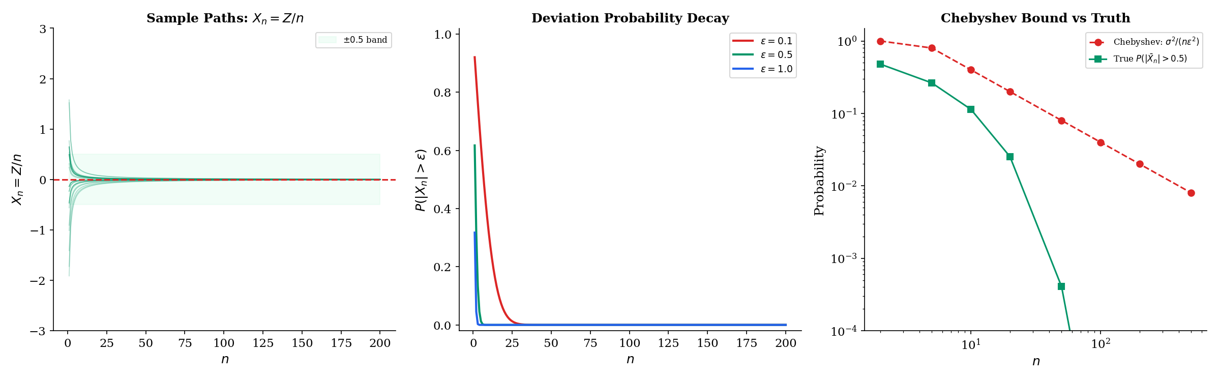
Let and define . We claim .
For any :
Since is standard Normal, we can bound this using the tail inequality for . So:
This decays exponentially fast to zero. For concrete values with :
| 1 | 0.1 | 0.920 |
| 5 | 0.5 | 0.617 |
| 10 | 1.0 | 0.317 |
| 50 | 5.0 | |
| 100 | 10.0 |
Notice that not only converges in probability — every single realization converges deterministically, since for each fixed , . So this sequence actually converges almost surely, which is stronger. The next section makes that distinction precise.
9.3 Almost Sure Convergence
Convergence in probability says: at any fixed time , the probability of being far from the target is small. Almost sure convergence says something much stronger: with probability 1, the entire sample path eventually settles near the target and stays there. The distinction matters. A sequence could converge in probability (deviations become rare) while occasionally producing large excursions that persist along every sample path — the typewriter sequence of Section 9.7 does exactly this.
A sequence converges almost surely (a.s.) to if
Equivalently, , meaning the set of sample points where the sequence of real numbers converges to has probability 1.
We write .
The critical difference from convergence in probability: a.s. convergence requires that for probability-1 many outcomes , there exists (depending on the outcome) such that for all . The quantifier structure is: , .
The definition involves , which in turn involves and . An equivalent characterization avoids the limit and works directly with tail events.
if and only if for every :
Equivalently, for every , where
is the event that infinitely often.
Proof [show]
We show both directions of the equivalence.
Forward direction. Suppose , so . The event — the set of where does not converge to — can be written as:
This is because means there exists some (which we can take to be for some integer ) such that for infinitely many .
Since and the union above covers :
for each . Since probabilities are non-negative, for every . For arbitrary , choose with ; then , so , and the result follows.
Now, the event . The sets are decreasing (), so by continuity of probability from above:
Since this equals 0, we have .
Reverse direction. Suppose for every . Then:
So , which is .
The Borel-Cantelli characterization reveals why a.s. convergence is harder to establish than convergence in probability. For convergence in probability, we only need each individual . For a.s. convergence, we need the supremum , which controls all future times simultaneously.
Let be iid with and . Then
This is the Strong Law of Large Numbers (SLLN). It says more than Theorem 9.1: not only does (which is convergence in probability), but with probability 1, the realized sequence converges to as a sequence of real numbers.
The SLLN is the justification for Monte Carlo simulation: when we estimate by averaging , the a.s. convergence guarantees that our single run of the simulation will produce an average that converges to the truth. Convergence in probability alone would only guarantee this “with high probability” — we’d need to worry about rare bad runs. The SLLN says those bad runs have probability zero.
The full proof requires Kolmogorov’s maximal inequality and a truncation argument — see Law of Large Numbers for the complete Etemadi proof. The key difficulty is controlling the supremum , which the Chebyshev argument of Theorem 9.1 cannot do.
The event is a tail event — it depends only on the “tail” of the sequence and is unaffected by changing any finite number of terms. Kolmogorov’s 0-1 law states that every tail event has probability either 0 or 1. So before we even prove the SLLN, we know that . The SLLN’s job is to establish that the answer is 1, not 0.
This 0-1 structure is why almost sure convergence results tend to be all-or-nothing: either the sample mean converges a.s. to the right thing, or it doesn’t converge a.s. at all. There’s no middle ground like “converges a.s. with probability 0.7.”
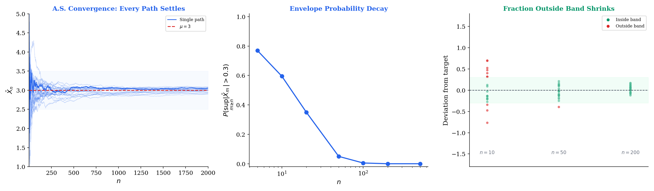
The interactive explorer below generates sample paths and lets you watch them converge (or not). Try switching between sequences that converge almost surely and sequences that converge only in probability — the difference is visible in the paths.
9.4 Convergence in
Almost sure convergence and convergence in probability are both qualitative — they measure whether is close to , but not how far away it is on average. convergence brings quantitative control: it requires that the -th moment of the gap vanishes.
For , a sequence converges in to if
We write . This requires that both and have finite -th moments.
The norm of a random variable is , so convergence is convergence in the norm: .
The most important special case is .
A sequence converges in mean square (or in ) to if
We write . Expanding the square:
So convergence requires both the variance of the gap and the squared bias to vanish. This is exactly the bias-variance decomposition applied to the “estimator” targeting the “parameter” .
convergence controls not just whether is close to , but whether the moments of approach those of .
If , then .
More generally, if and , then .
Proof [show]
Convergence of moments. We use Minkowski’s inequality (the triangle inequality for the norm):
and similarly , so:
Since means , we get , which is . Taking -th powers (the function is continuous on ) gives .
Higher implies lower . For , Jensen’s inequality (Topic 4, Theorem 13) applied to the convex function gives:
Taking the -th root of both sides:
So implies . In particular, convergence implies convergence.
This theorem highlights an important contrast. Convergence in probability does not guarantee convergence of moments (Example 7 in Section 9.7 will show this dramatically). convergence does — it’s what you need when moment control matters, which is most of statistics.
Let and define . We claim .
We compute directly:
So , confirming convergence. The rate of convergence is — quite fast.
For comparison, , which also goes to zero. Both the bias and the variance vanish, as required by the bias-variance decomposition of .
![Lp norms E[|Xn - X|^p] decaying to zero for p = 1, 2, and 4](/images/topics/modes-of-convergence/lp-convergence.png)
9.5 Convergence in Distribution
The three modes above all require the random variables and to live on the same probability space — they compare the random variables pointwise (a.s.), moment-wise (), or event-wise (in probability). Convergence in distribution breaks free of this requirement. It compares only the distributions of and , which can live on entirely different probability spaces.
This is the weakest mode, but it’s also the most important for asymptotic statistics. The Central Limit Theorem — the single most-used result in statistical inference — is a statement about convergence in distribution.
A sequence converges in distribution to if
at every point where is continuous. We write .
The restriction to continuity points of is essential. At jump points of , the CDFs may converge to a value different from due to the discontinuity. For instance, if (a deterministic sequence converging to 0) and , then for all but . At — a discontinuity of — the CDFs do not converge. But at every other , they do.
Convergence in distribution is sometimes called weak convergence or convergence in law. The notation and are also common.
The most powerful characterization of convergence in distribution comes from the Portmanteau lemma, which gives five equivalent conditions.
The following are equivalent:
(i) at every continuity point of .
(ii) for every bounded continuous function .
(iii) for every open set .
(iv) for every closed set .
(v) for every Borel set with (where is the boundary of ).
Proof [show]
We prove the implication (i) (ii), which is the direction most often used in practice.
Assume at all continuity points of , and let be a bounded continuous function with .
Fix . Since is a CDF, it has at most countably many discontinuities. Choose such that both and are continuity points of and and . This is possible because as and as , and the discontinuity set is countable.
On the compact interval , the continuous function is uniformly continuous. So there exists such that whenever .
Partition into subintervals with mesh , choosing each to be a continuity point of (again possible since discontinuities are countable).
For each subinterval , the value of varies by at most from . So the step function satisfies for .
Now we bound . Split the expectation into three parts — the tails and , and the middle :
For the tail terms, since :
Since is a continuity point of , , so for large , . Similarly for the right tail. Combined, the tail contributions are at most for both and .
For the middle term, replace with at cost . The expectation of depends only on for each , and since all are continuity points of , these converge to . So for large enough , the step-function expectations are within .
Combining: for all sufficiently large , . Since was arbitrary, .
Characterization (ii) — convergence of expectations of bounded continuous functions — is the one most frequently used in proofs. It’s the definition of weak convergence in functional analysis, which is why convergence in distribution is also called “weak convergence.”
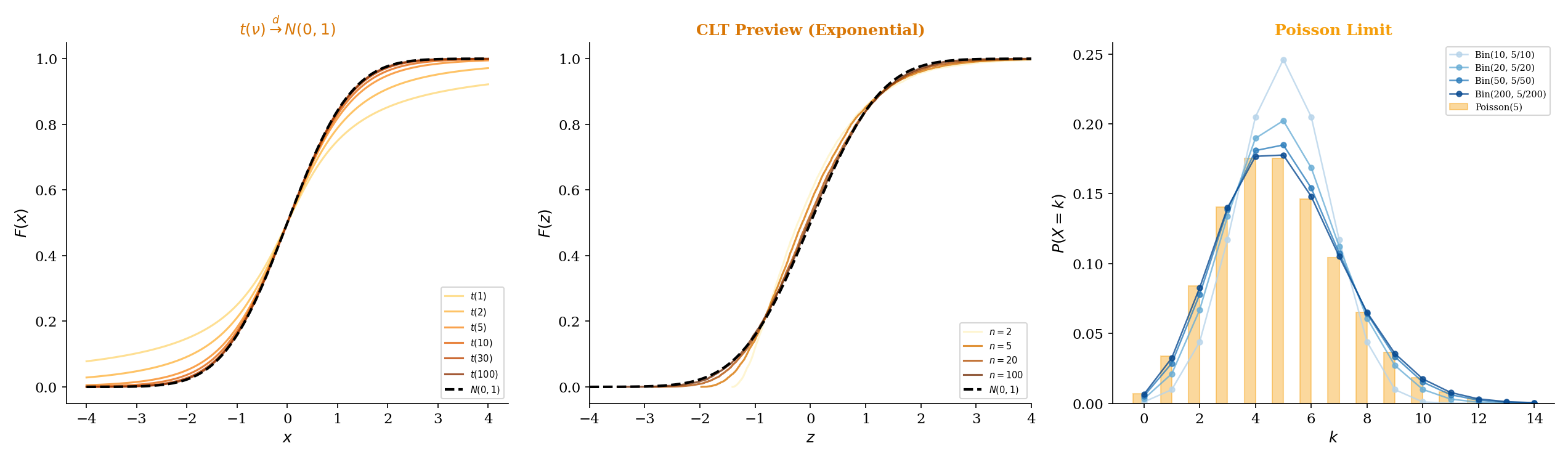
As previewed in Topic 6 — Continuous Distributions (Theorem 18), the Student’s distribution with degrees of freedom converges in distribution to the standard Normal:
Recall that where and are independent. By the law of large numbers applied to the chi-squared (which is a sum of independent squared Normals), . So by the continuous mapping theorem (Theorem 9.9, Section 9.8).
The punchline is Slutsky’s theorem (Theorem 9.10, Section 9.8): if (trivially) and , then .
This is why, for large , the -distribution and the Normal give nearly identical critical values. At , the 97.5th percentile of is 2.042 versus 1.960 for the Normal — a difference of about 4%.
If the moment-generating functions converge to for all in an open interval containing 0, and is the MGF of some distribution, then .
This is the MGF version of Levy’s continuity theorem (the full version uses characteristic functions, which always exist). It converts a convergence-in-distribution problem into a pointwise limit of MGFs — a calculus problem rather than a probability problem. This is exactly the technique we’ll use to prove the Poisson limit theorem (Section 9.9) and the Central Limit Theorem.
The MGF version requires that the limit MGF exists in a neighborhood of 0. When it does, MGF uniqueness (Topic 4, Theorem 17) identifies the limiting distribution. The characteristic function version avoids this existence requirement, which is why the full CLT proof uses characteristic functions for the most general version.
9.6 The Convergence Diamond
We now have all four modes. The natural question: how do they relate? The answer is a diamond-shaped implication diagram with almost sure and at the top, convergence in probability in the middle, and convergence in distribution at the bottom. The arrows point downward — each mode implies the ones below it, but the reverse implications fail.
Convergence Hierarchy
We prove each arrow in the diamond.
If , then .
Proof [show]
Fix . Define the indicator random variable . We need to show .
Since , for almost every , . This means for almost every , so for almost every . That is, almost surely.
Now, for all (since is an indicator), so is bounded by the constant function 1, which is integrable. By the bounded convergence theorem (a special case of the dominated convergence theorem):
Therefore , which is .
If for some , then .
Proof [show]
This is a direct application of Markov’s inequality (Topic 4, Theorem 11). Fix . Apply Markov’s inequality to the non-negative random variable with threshold :
Since , the numerator . The denominator is a fixed positive constant. So:
By the squeeze theorem, .
If , then .
Proof [show]
Fix a continuity point of . We need to show .
Upper bound. For any :
The first term: if and , then , so:
The second term is at most . Combining:
Lower bound. Similarly:
If and , then , so:
Therefore:
Rearranging: .
Combining the bounds:
Now take . Since , . So:
This holds for every . Now take . Since is a continuity point of , both and . By the squeeze:
So , which is .
There is one partial converse worth knowing: convergence in probability implies a.s. convergence along a subsequence.
If , then there exists a subsequence such that .
Proof [show]
Since , for each integer , as . So we can choose (with ) such that:
Define the events . Then:
By the first Borel-Cantelli lemma, . That is, with probability 1, only finitely many of the events occur. So for almost every , there exists such that for all :
Since , this gives for almost every , which is .
This subsequence result is a key technical tool. It’s how most proofs upgrade convergence in probability to almost sure convergence: extract a subsequence that converges a.s., use the a.s. convergence to establish some property, then extend back to the full sequence.
The mode of convergence you need depends on what you’re trying to do:
-
Almost sure convergence is what you need for SGD guarantees. When training a neural network, you run one optimization trajectory. The SLLN (a.s. convergence of the sample mean) and Robbins-Monro theory (a.s. convergence of SGD iterates) guarantee that your specific run converges — not just that runs converge “on average” or “with high probability.”
-
Convergence in probability is what PAC learning provides. A PAC bound says — the empirical risk is close to the true risk with probability at least . This is convergence in probability, not a.s. You can’t guarantee that every dataset will give a good estimate, but the bad datasets become vanishingly rare.
-
Convergence in distribution is what the CLT gives. The statement tells you the shape of the sampling distribution is approximately Normal. It says nothing about individual sample paths converging — only about the aggregate distributional behavior. This is enough for confidence intervals and hypothesis tests.
Choosing the wrong mode is like using a wrench as a hammer — it might work, but you lose the guarantee. If you need every training run to converge, convergence in distribution is insufficient. If you need the distribution of a test statistic, a.s. convergence is overkill.
9.7 Counterexamples: Why the Arrows Don’t Reverse
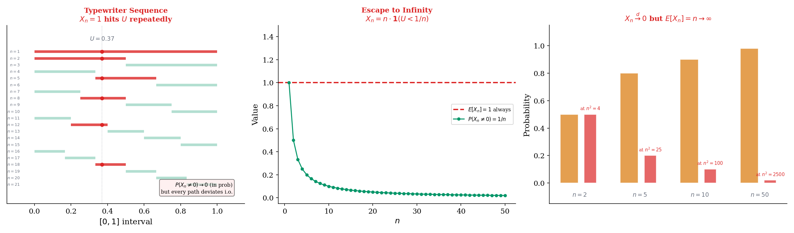
The hierarchy in Section 9.6 has three missing arrows: in probability does not imply a.s., in probability does not imply , and convergence in distribution does not imply convergence of expectations. We now construct explicit counterexamples for each.
Let . We construct a sequence that converges to 0 in probability but not almost surely. The idea: let intervals of decreasing length “slide” across repeatedly, so every point gets covered infinitely often.
Construction. Index the sequence so that for the -th pass, we divide into equal intervals, each of length . The first pass () has one interval . The second pass () has two intervals and . The third pass () has three intervals , , . And so on.
Formally, we define a mapping from to a pair where is the pass number and is the interval within that pass. The relationship is: (since the first passes use indices). Then:
Convergence in probability. For each in pass , . Since as (specifically, ), we have for any . So .
Failure of a.s. convergence. Fix any . In pass , the point falls in the interval . So for the index corresponding to , we have . This happens for every , so for infinitely many . Since for other in the same pass, the sequence oscillates between 0 and 1 forever and does not converge.
This holds for every , so . Not only does the sequence fail to converge a.s. to 0 — it fails to converge a.s. to anything.
Let and define:
Convergence in probability. . So for any , , giving .
Failure of convergence. The expected value is:
for every . So . We do not have .
The intuition: as grows, is nonzero with vanishing probability (convergence in probability), but when it is nonzero, its value is — growing without bound. The spike becomes less likely but taller, maintaining a constant expectation. The probability mass that “escapes to infinity” prevents convergence.
More dramatically, , so we don’t have convergence either. The sequence converges in probability but in no space.
Define by:
Convergence in distribution. The CDF of is: for , for , and for .
For any fixed , once is large enough that , we have (where is the CDF of the constant 0: ). For , trivially. So .
Divergence of expectations. But:
The distributions converge to a point mass at 0, yet the expectations diverge to infinity. The tiny probability mass at is invisible to the CDF at any fixed , but it dominates the expectation.
This is why convergence in distribution — the mode the CLT provides — does not automatically give convergence of moments. For the CLT, the moments of do converge to those of , but this requires additional uniform integrability arguments beyond the basic convergence-in-distribution statement.
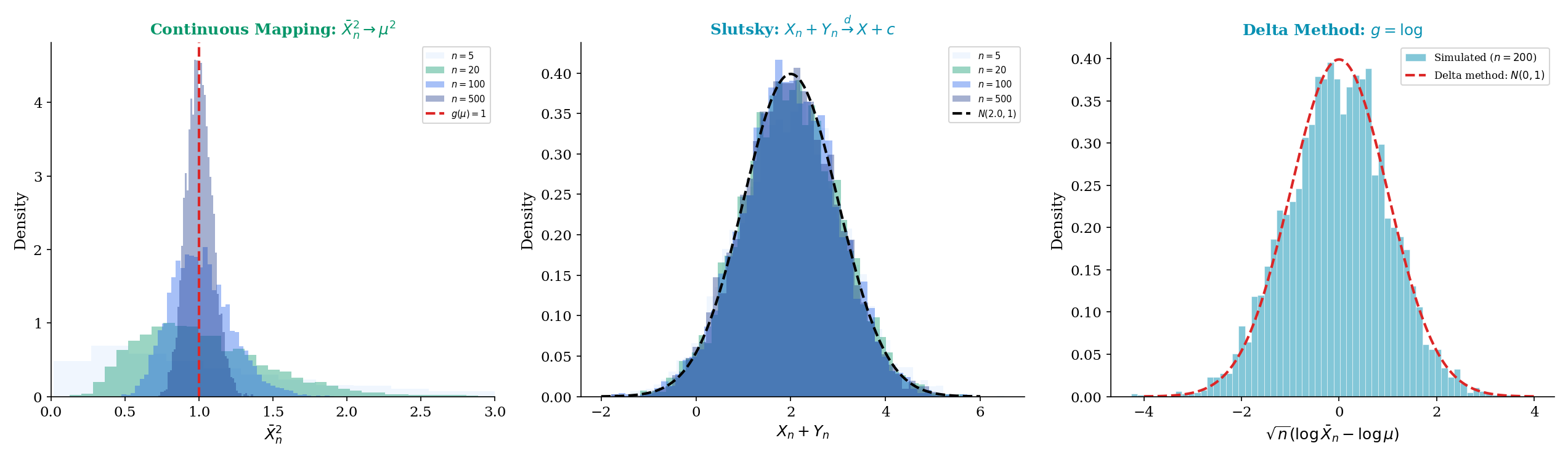
9.8 Continuous Mapping, Slutsky, and the Delta Method
The four modes of convergence tell us how sequences of random variables approach their limits. But in practice, we rarely work with the raw sequence — we transform it, combine it with other sequences, and apply functions. The continuous mapping theorem, Slutsky’s theorem, and the delta method are the three tools that let us do this while preserving convergence guarantees.
Let be a continuous function. Then:
(a) If , then .
(b) If , then .
(c) If , then .
In short, continuous functions preserve all three modes of convergence.
Proof [show]
We prove part (b) in full, which illustrates the key technique.
Fix . We need to show .
The difficulty is that is continuous on all of , but continuity only gives us local control: for each , if is close to , then is close to . On a compact set, this local control becomes uniform. On all of , we need to handle the tails separately.
Step 1: Truncation. Choose large enough that . This is possible because as .
Step 2: Uniform continuity on compact sets. On the compact set , the continuous function is uniformly continuous. So there exists (with ) such that whenever and both .
Step 3: Event decomposition. We split:
To see why: if , , and , then both and lie in and , so by uniform continuity. The contrapositive gives the inclusion above.
Step 4: Bounding each piece.
The first term because .
The second term by our choice of .
The third term: (triangle inequality), so . The first part goes to 0 (convergence in probability), and the second is at most .
Combining, for all sufficiently large :
Since was arbitrary, , giving .
The continuous mapping theorem handles transformations of a single converging sequence. Slutsky’s theorem handles combinations of a converging-in-distribution sequence with a converging-in-probability sequence.
If and (where is a constant), then:
(a)
(b)
(c) provided
Proof [show]
We prove part (a). Parts (b) and (c) follow by similar arguments.
We use the Portmanteau characterization (Theorem 9.4, part (ii)): we need to show for every bounded continuous .
Let be bounded by and continuous. Fix . Since is continuous and bounded, it is uniformly continuous on any compact set. Choose large enough that and for all large (the latter follows from convergence in distribution via tightness).
On , is uniformly continuous: there exists such that when and both .
Now decompose:
Split this expectation based on whether and :
When and : both and lie in (for ), and , so .
On the complementary event:
Since , . By tightness, for large . So for large :
Now, the continuous mapping theorem for convergence in distribution (applied to , which is bounded and continuous) gives .
Combining: for large . Since was arbitrary and was an arbitrary bounded continuous function, by the Portmanteau lemma.
Slutsky’s theorem is the workhorse of asymptotic statistics. It’s how we derived in Example 4: the numerator converges in distribution to (trivially — it is ), the denominator converges in probability to 1, so the ratio converges in distribution to .
A crucial restriction: Slutsky’s theorem requires one of the two sequences to converge to a constant. If both and converge in distribution to non-degenerate limits, the joint behavior of is not determined by the marginal limits — we would need information about the joint distribution.
The delta method converts a convergence-in-distribution result about into one about , with explicit variance formulas.
Suppose , and let be a function that is differentiable at with . Then:
In words: the asymptotic variance of is times the asymptotic variance of .
The proof uses a Taylor expansion and Slutsky’s theorem. The key insight is that for close to , , so the distribution of is approximately times the distribution of .
When , the first-order Taylor term vanishes and we need the second-order term.
Suppose , and let be twice differentiable at with and . Then:
Note the scaling changes from to : the convergence rate is slower when the first derivative vanishes.
Let be iid with mean and variance . By the CLT (proved in full in Topic 11):
Apply the delta method with . We have , so (since ). Therefore:
The asymptotic variance of is .
Concrete computation for Exponential(1). If , then and . The delta method gives:
So has asymptotic variance — exactly the same as itself in this special case. This is because , so the log transform preserves the asymptotic variance at .
For , the delta method variance is the squared coefficient of variation of the underlying distribution times . The coefficient of variation is dimensionless, which is why the log transform is natural for data with a constant CV (multiplicative noise models).
| Quantity | Delta Method | Simulation |
|---|---|---|
| Mean of g(X̄) | 1.6094 | 1.6073 |
| Variance of g(X̄) | 0.0016 | 0.0016 |
| μ | 5.0000 | |
| σ² | 4.0000 | |
| g(μ) | 1.6094 | |
| g′(μ) | 0.2000 | |
| [g′(μ)]² σ² / n | 0.0016 | |
9.9 Making the Poisson Limit Theorem Rigorous
In Topic 5 — Discrete Distributions, we stated that as . At the time, we verified this by showing the PMFs converge pointwise. Now we can make this fully rigorous using convergence in distribution, proved via MGF convergence (Levy’s continuity theorem, Remark 2).
Let for a fixed . Then:
Proof [show]
We prove this by showing that the MGF of converges to the MGF of at every , then invoking Levy’s continuity theorem (Remark 2).
Step 1: MGF of . The MGF of a random variable is (derived by exponentiating the binomial PMF and recognizing the binomial theorem). With :
Factor out the 1 and rewrite:
Step 2: Take the limit. This is a sequence of the form where . Since does not depend on (it depends only on and ), we can use the fundamental limit directly:
To be more careful, take the logarithm:
Using the Taylor expansion with :
As :
Exponentiating: .
Step 3: Identify the limit. The MGF of is:
So for all . The limit exists for all and is the MGF of .
Step 4: Apply Levy’s continuity theorem. Since converges to pointwise on all of (which contains a neighborhood of 0), and is the MGF of , the theorem gives .
By MGF uniqueness (Topic 4, Theorem 17), the limiting distribution is uniquely identified as .
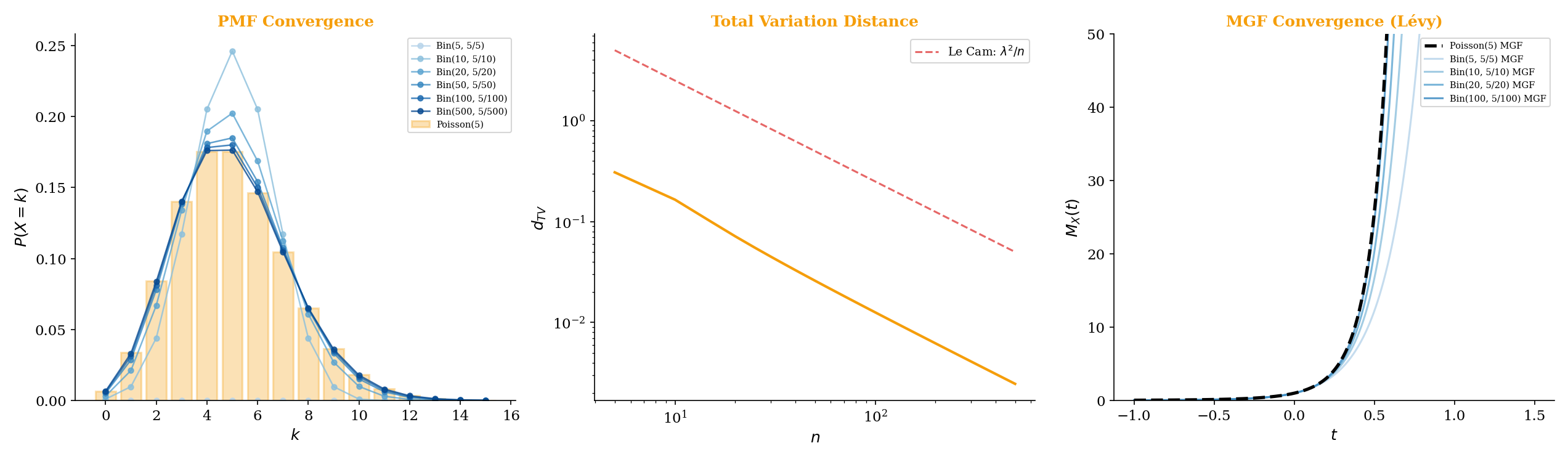
This proof is the prototype for the Central Limit Theorem proof. The technique is identical: compute the MGF, show pointwise convergence to the target MGF, and invoke Lévy’s continuity theorem. The CLT proof is more involved because the MGF of requires a careful Taylor expansion of , but the structure established here carries over directly.
9.10 Connections to Machine Learning
The four modes of convergence are not abstract curiosities — they appear throughout machine learning, often implicitly. Recognizing which mode is at play helps you understand what a convergence guarantee actually promises and what it leaves open.
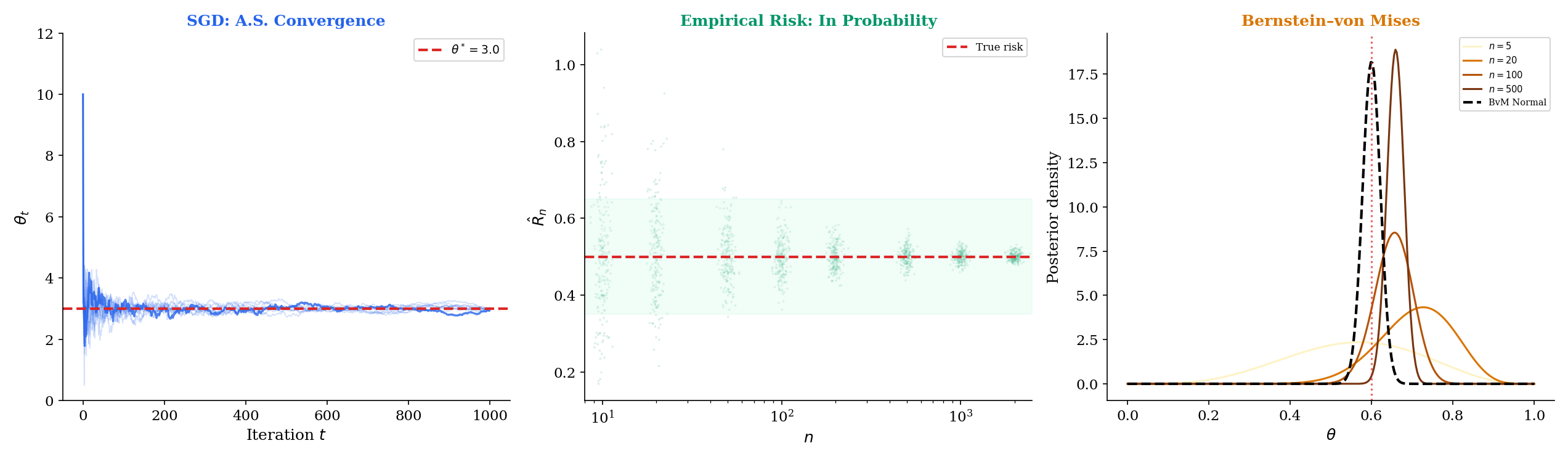
Scenario 1: SGD with Robbins-Monro step sizes (almost sure convergence).
Consider stochastic gradient descent on a loss function with updates , where is a random minibatch and is the step size. The Robbins-Monro conditions require:
The first condition ensures the step sizes are large enough to reach any minimum. The second ensures they decay fast enough that the noise averages out. Under these conditions (plus regularity assumptions on ), the iterates , a local minimum.
Why almost sure convergence matters: you run SGD once. A single training run produces a single trajectory Almost sure convergence guarantees that this specific trajectory converges — not just that “most” trajectories converge.
With a constant step size (common in practice for speed), the Robbins-Monro conditions fail (). The iterates then converge only in probability to a neighborhood of , with the neighborhood size proportional to . This is the exploration-exploitation tradeoff made explicit through convergence modes.
Scenario 2: PAC learning (convergence in probability).
In Probably Approximately Correct (PAC) learning, the fundamental guarantee has the form:
where is the true risk of hypothesis , is the empirical risk on training samples, and decreases with . This is convergence in probability: with high probability, the empirical risk is close to the true risk.
The “sup over ” makes this a uniform convergence statement — the empirical risk concentrates simultaneously for all hypotheses in the class. The rate at which depends on the complexity of (VC dimension, Rademacher complexity), and this rate is what distinguishes learnable from unlearnable hypothesis classes.
Scenario 3: Bernstein-von Mises theorem (convergence in distribution).
In Bayesian statistics, the posterior distribution for a parameter given iid observations satisfies:
where is the Fisher information at the true parameter . This is convergence in distribution: the posterior shape approaches a Normal, regardless of the prior (under regularity conditions).
This is the frequentist justification for Bayesian inference: with enough data, the posterior is approximately Normal centered at the MLE, and the prior washes out. The convergence is in distribution — we’re comparing the posterior distribution to the Normal, not individual samples or paths.
Knowing that a sequence converges is useful, but knowing how fast it converges is essential for practice. The modes of convergence defined in this topic are qualitative — they say whether the limit is reached, not how quickly.
Convergence rates quantify the speed:
-
Hoeffding’s inequality gives exponential decay for convergence in probability: for bounded random variables in . This is much sharper than the rate from Chebyshev.
-
The Berry–Esseen theorem gives the rate for convergence in distribution in the CLT: , where . The CLT convergence rate is .
-
Large deviations theory characterizes the exponential rate at which decays for sets that are far from the mean. The rate function is the Fenchel-Legendre transform of the log-MGF.
These rate results are the subject of Large Deviations & Tail Bounds. They bridge the gap between the existence of convergence (this topic) and the speed of convergence (which determines sample size requirements in practice) — Hoeffding, Bernstein, and the Cramér rate function quantify exactly how fast convergence occurs.
9.11 Summary
This topic defined the four modes of convergence for sequences of random variables, established the implication hierarchy between them, and built the tools — continuous mapping, Slutsky, delta method — for working with convergent sequences in practice.
The Four Modes
| Mode | Definition | Intuition | Guarantees | Does NOT Guarantee | ML Application |
|---|---|---|---|---|---|
| Almost sure | Every path settles | Path-by-path convergence | Moment convergence | SGD convergence | |
| Average -th gap vanishes | Moment convergence | Path-by-path convergence | MSE-consistent estimation | ||
| In probability | Deviations become rare | Subsequential a.s. convergence | Full a.s. convergence, moment convergence | PAC learning bounds | |
| In distribution | CDFs approach | Shape convergence | Moment convergence, path convergence | CLT, asymptotic tests |
The Convergence Diamond
Almost sure and are incomparable — neither implies the other in general.
The Tools
- Continuous mapping (Theorem 9.9): continuous functions preserve all modes.
- Slutsky (Theorem 9.10): convergence in distribution + convergence in probability to a constant = convergence in distribution.
- Delta method (Theorems 9.11-9.12): transforms CLT-type results through differentiable functions.
- MGF convergence (Remark 2): pointwise convergence of MGFs implies convergence in distribution.
Formal Element Index
| Element | Name | Section |
|---|---|---|
| Definition 9.1 | Convergence in probability | 9.2 |
| Definition 9.2 | Consistency | 9.2 |
| Definition 9.3 | Almost sure convergence | 9.3 |
| Definition 9.4 | convergence | 9.4 |
| Definition 9.5 | Mean square convergence | 9.4 |
| Definition 9.6 | Convergence in distribution | 9.5 |
| Theorem 9.1 | Sample mean convergence (WLLN preview) | 9.2 |
| Theorem 9.2 | Borel-Cantelli characterization | 9.3 |
| Theorem 9.3 | implies moment convergence | 9.4 |
| Theorem 9.4 | Portmanteau lemma | 9.5 |
| Theorem 9.5 | A.s. implies in probability | 9.6 |
| Theorem 9.6 | implies in probability | 9.6 |
| Theorem 9.7 | In probability implies in distribution | 9.6 |
| Theorem 9.8 | In probability implies a.s. along subsequence | 9.6 |
| Theorem 9.9 | Continuous mapping theorem | 9.8 |
| Theorem 9.10 | Slutsky’s theorem | 9.8 |
| Theorem 9.11 | Delta method (first order) | 9.8 |
| Theorem 9.12 | Delta method (second order) | 9.8 |
| Theorem 9.13 | Poisson limit theorem | 9.9 |
What Comes Next
This topic established the modes of convergence — the different senses in which sequences of random variables can approach a limit. The next three topics apply these modes to the three pillars of asymptotic probability:
-
Law of Large Numbers: The WLLN proves under finite variance (Theorem 10.1) and under finite mean alone (Khintchine, Theorem 10.3). The SLLN proves under finite mean alone (Etemadi, Theorem 10.5). The Glivenko–Cantelli theorem proves uniform a.s. convergence of the empirical CDF.
-
Central Limit Theorem: The CLT proves (convergence in distribution). The proof via MGF convergence follows the same technique we used for the Poisson limit theorem in Section 9.9. The Lindeberg CLT extends the result to non-identical summands, and the Berry–Esseen theorem quantifies the convergence rate.
-
Concentration Inequalities: While the CLT gives the shape of the limiting distribution, concentration inequalities give rates — how fast the convergence happens. Hoeffding, Bernstein, and sub-Gaussian tail bounds provide the exponential-rate guarantees that power finite-sample statistical learning theory — PAC bounds, Rademacher complexity, and sample complexity calculations.
References
- Billingsley, P. (2012). Probability and Measure (Anniversary ed.). Wiley.
- Durrett, R. (2019). Probability: Theory and Examples (5th ed.). Cambridge University Press.
- Casella, G. & Berger, R. L. (2002). Statistical Inference (2nd ed.). Duxbury.
- Resnick, S. (2014). A Probability Path. Birkhäuser.
- Wasserman, L. (2004). All of Statistics. Springer.
- Bishop, C. M. (2006). Pattern Recognition and Machine Learning. Springer.