Conditional Probability & Independence
How new information reshapes probability — from Bayes' theorem to the conditional independence assumption that makes probabilistic ML tractable
1. Conditional Probability
In Topic 1 we built the machinery of probability spaces: sample spaces, sigma-algebras, and the Kolmogorov axioms. Everything there describes unconditional probability — the probability of events in the absence of any additional information.
But in practice, we almost always have partial information. A doctor knows the patient tested positive before computing the probability of disease. A spam filter knows the email contains the word “lottery” before computing the probability it’s spam. A stock trader knows yesterday’s return before estimating today’s. The question becomes: how does knowing that occurred change the probability of ?
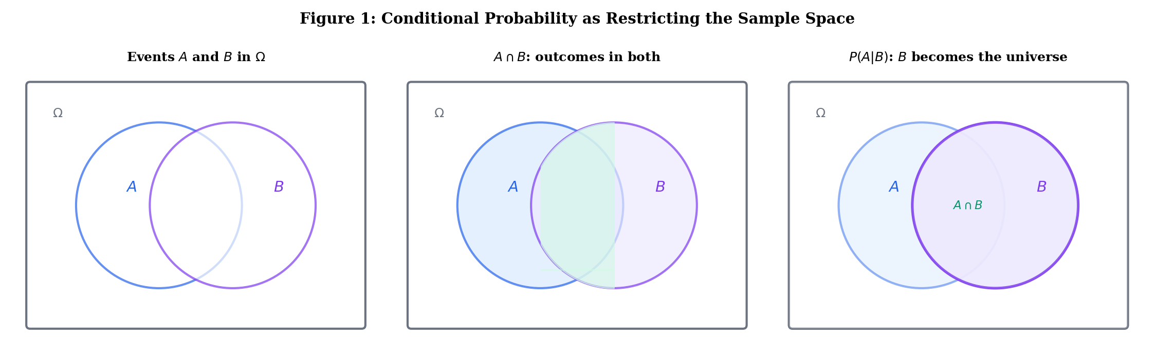
Let be a probability space and let with . The conditional probability of given is
The intuition is clean: conditioning on means restricting our universe to outcomes in . Among those outcomes, we ask how many also belong to . The denominator re-normalizes so that — the new “sample space” has total probability 1.
Roll a fair die, with . Let (even) and (at least 4).
Knowing the roll was at least 4, the probability of even jumps from to . Information changed the probability.
For fixed with , the function satisfies the Kolmogorov axioms on :
- (non-negativity).
- (normalization).
- Countable additivity follows from that of .
So conditioning on gives us a new probability space — the same and , but a different measure. Every theorem we proved in Topic 1 (complement rule, inclusion-exclusion, union bound, continuity) holds for conditional probabilities too.
For with , define by . Then is a probability space.
Use the explorer below to see how conditioning on restricts the sample space and reshapes probabilities. Toggle “Condition on B” to watch fade and become the new universe:
2. The Multiplication Rule and Chain Rule
The Multiplication Rule
Rearranging the definition of conditional probability gives us the multiplication rule (also called the product rule):
For events with ,
By symmetry (when ): .
Proof Multiplication Rule [show]
Multiply both sides of by . ∎
This is trivial as a proof, but powerful as a computational tool. It converts a joint probability into a conditional probability times a marginal — and often the conditional is the easier quantity to reason about.
The Chain Rule
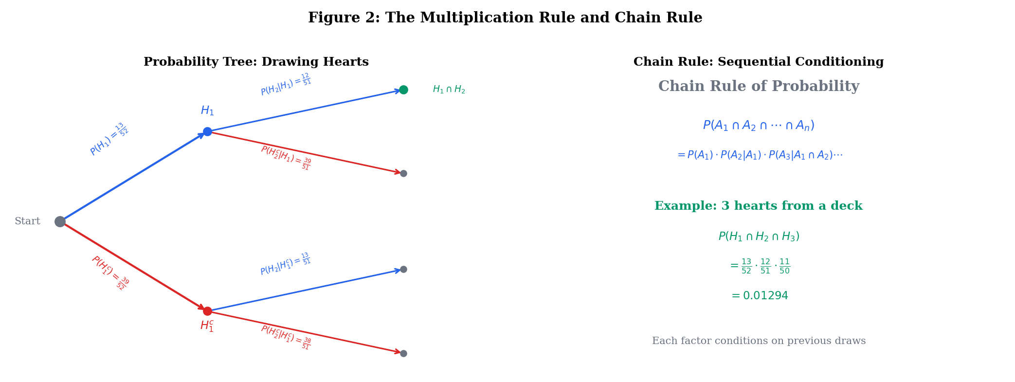
Applying the multiplication rule repeatedly gives the chain rule of probability:
For events with ,
The proof is a straightforward induction using the multiplication rule at each step: the base case is Theorem 1, and the inductive step applies the multiplication rule to and .
Draw 3 cards from a standard 52-card deck without replacement. What is the probability all three are hearts?
Each factor reflects the updated state of the deck: after drawing one heart, 12 of 51 remaining cards are hearts. The chain rule captures this sequential conditioning perfectly.
Why this matters for ML: The chain rule is the foundation of autoregressive models. A language model factorizes — this is exactly the chain rule applied to a sequence of token events.
3. The Law of Total Probability
The law of total probability is one of the most useful results in all of probability. It lets us compute by “dividing and conquering” — breaking the computation into cases.
Let be a partition of : the are pairwise disjoint and . If for all , then for any event ,
Proof Law of Total Probability [show]
Since the partition , we have . The sets are pairwise disjoint (because the are). By countable additivity:
where the last step uses the multiplication rule. ∎
The most common application uses a two-element partition :
A disease has 2% prevalence. A test has sensitivity and specificity . What is , the probability of testing positive?
Partition: . By total probability:
About 11.7% of people test positive — and the vast majority are false positives, because the disease is rare. This is where Bayes’ theorem comes in.
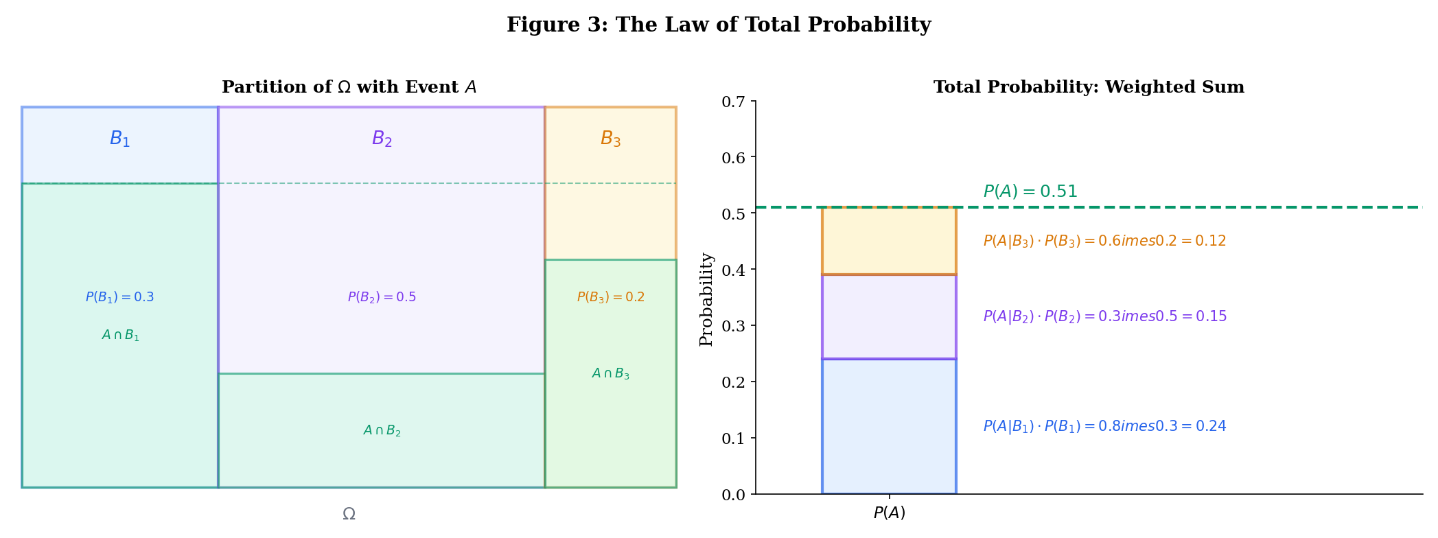
Use the explorer below to partition into 2, 3, or 4 regions and see how the law of total probability decomposes into weighted contributions:
4. Bayes’ Theorem
Bayes’ theorem is the multiplication rule used twice, combined with total probability. It answers: given that we observed , what is the probability that it was caused by (or associated with) ?
Let with and . Then
More generally, if partition with for all , then
Proof Bayes' Theorem [show]
By the multiplication rule, . Divide by :
The general form follows by expanding via the law of total probability. ∎
The Bayesian Vocabulary
Bayes’ theorem has a canonical interpretation:
| Term | Symbol | Role |
|---|---|---|
| Prior | Probability of before observing | |
| Likelihood | Probability of the evidence given | |
| Evidence | Total probability of (normalization constant) | |
| Posterior | Probability of after observing |
In shorthand: posterior likelihood prior. The evidence is just the normalizing constant that makes the posterior sum to 1.
Humans are notoriously bad at Bayesian reasoning. We tend to overweight the likelihood and ignore the prior — the base rate. In medical testing, this means patients (and sometimes doctors) confuse “the test is 99% accurate” with “I’m 99% likely to have the disease.” As Example 4 shows, these can be wildly different when the disease is rare.
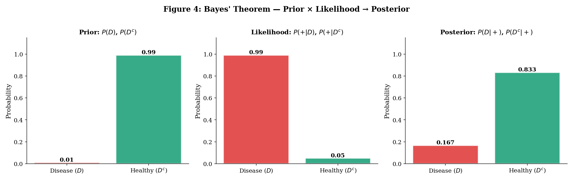
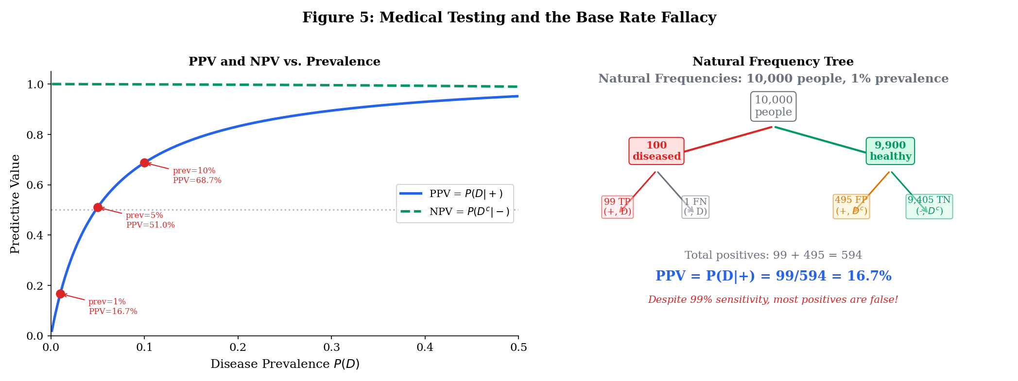
The Medical Testing Example
A disease has prevalence (1% of the population). A diagnostic test has:
- Sensitivity: (catches 99% of true cases)
- Specificity: (correctly clears 95% of healthy people), so .
Question: If you test positive, what is the probability you actually have the disease?
By Bayes:
Despite a “99% accurate” test, a positive result means only about a 17% chance of disease. The base rate (1% prevalence) dominates.
Natural frequency framing. Consider 10,000 people:
- 100 have the disease → 99 test positive (true positives), 1 tests negative (false negative)
- 9,900 are healthy → 495 test positive (false positives), 9,405 test negative (true negatives)
- Total positives: 99 + 495 = 594. Of those, 99 actually have the disease: .
Explore Bayes’ theorem interactively below. Try the medical testing presets to see how PPV changes dramatically with prevalence — even when sensitivity and specificity stay fixed:
We start with our prior beliefs: P(A) and P(Aᶜ), which must sum to 1.
5. Independence
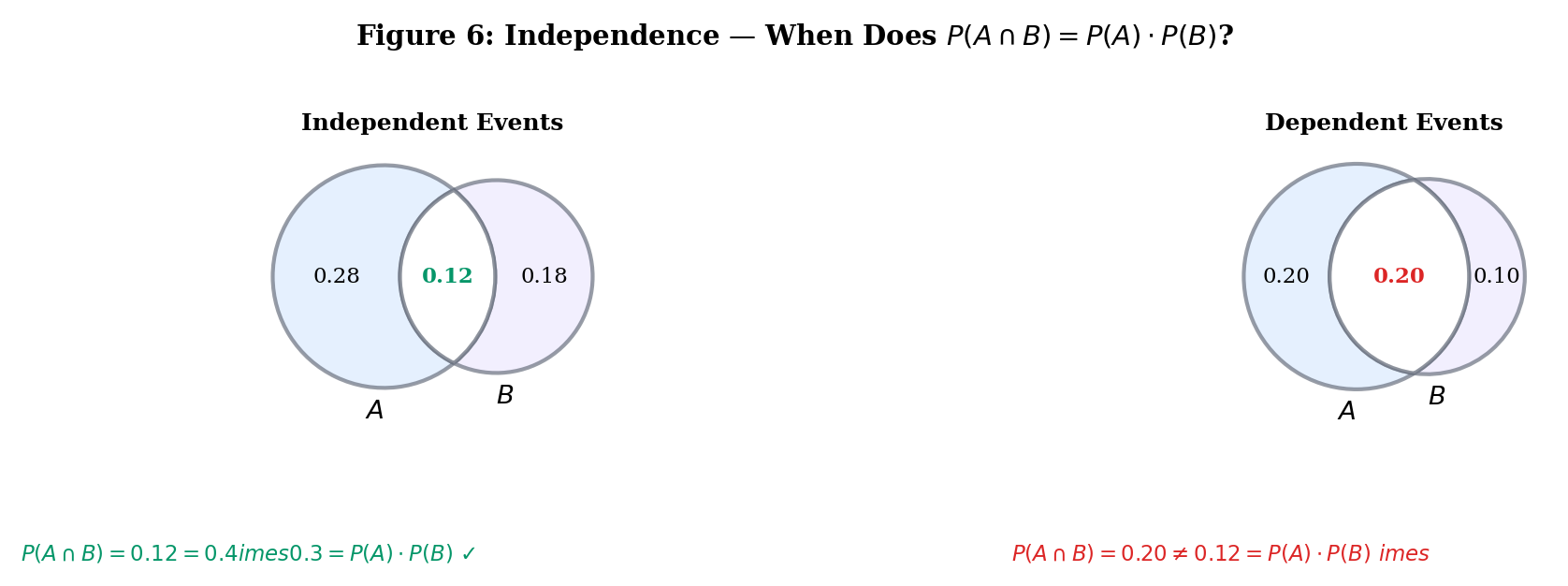
Two events are independent when knowing one occurred gives no information about the other. The formal definition says this in the most computationally useful way:
Events and are independent if
Equivalently (when ): — conditioning on doesn’t change the probability of .
Flip two fair coins. Let = “first coin is heads” and = “second coin is heads.” Then with .
Independent. This matches our intuition: the second coin doesn’t “know” what the first coin did.
Events are (mutually) independent if for every subset with ,
This requires conditions — not just the pairwise ones. For three events, we need four conditions: the three pairwise ones plus .
Independence of Complements
If and are independent, then and are also independent (and and , etc.).
Proof Independence of Complements [show]
We need to show .
The first equality uses with the two sets disjoint. The second uses the independence assumption .
This is reassuring: if “rain” and “traffic jam” are independent, then “no rain” and “traffic jam” should be too.
Use the tester below to build events on a die and check whether they’re independent. Try the presets, then define your own:
6. Pairwise vs. Mutual Independence
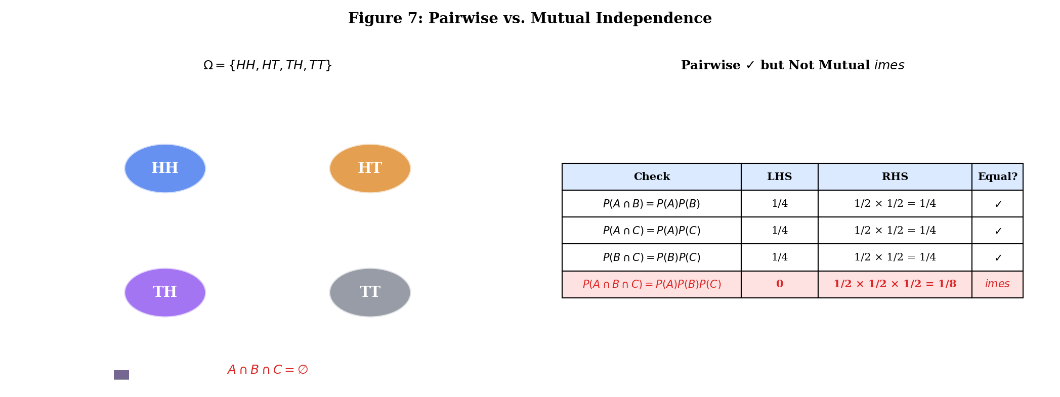
Pairwise independence — checking for all pairs — does not guarantee mutual independence. You also need the higher-order conditions.
Events are pairwise independent if for all .
Flip two fair coins. Define:
- = “first coin is heads”:
- = “second coin is heads”:
- = “the two coins show different faces” :
Check pairwise independence:
- ✓
- ✓
- ✓
But (both heads means same face, so fails), so:
The three events are pairwise independent but not mutually independent.
This is not a pathological edge case. In machine learning, pairwise decorrelation (e.g., PCA) does not guarantee full independence — a fact that higher-order methods like ICA (independent component analysis) exploit. The difference between pairwise and mutual independence is the difference between matching second-order statistics and matching the full joint distribution.
7. Conditional Independence
Conditional independence is arguably the most important concept in probabilistic ML. It says: “once we know , and become independent.”
Events and are conditionally independent given (written ) if
Equivalently (when ): — once you know , learning tells you nothing new about .
Independence Does NOT Imply Conditional Independence
This is the subtle part. All four combinations are possible:
| Marginally independent? | Conditionally independent given ? | Name |
|---|---|---|
| Yes | Yes | Fully independent |
| Yes | No | Explaining away (Berkson’s paradox) |
| No | Yes | Confounding |
| No | No | Generally dependent |
There exist events , , such that (marginally independent) but and are not conditionally independent given . And vice versa.
Proof Conditional Independence Does Not Imply Marginal Independence [show]
By construction. The “explaining away” and “confounding” presets in the explorer below provide concrete probability distributions witnessing each direction. ∎
Two independent causes and can produce an effect . Marginally, . But conditioning on (the effect having occurred) makes and dependent: if we know the effect happened and didn’t cause it, becomes more likely. This is called explaining away.
Concrete example: A fire alarm () can be triggered by a fire () or by cooking smoke (). Fire and cooking smoke are independent events. But given that the alarm is ringing, learning there’s no fire makes cooking smoke more probable.
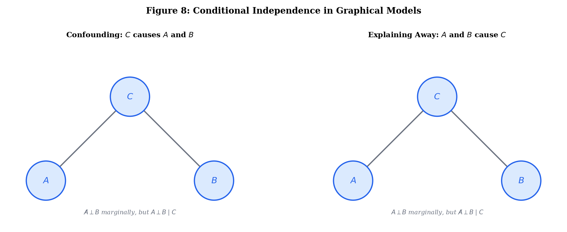
Conditional independence is the language of graphical models:
- In a Bayesian network (directed graph), is encoded by the graph structure (d-separation).
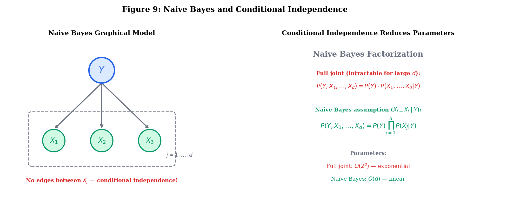
- The naive Bayes classifier assumes all features are conditionally independent given the class label: .
- In hidden Markov models, observations are conditionally independent given the hidden state.
These assumptions are rarely exactly true, but they make inference tractable. The art of probabilistic modeling is choosing which conditional independencies to assume.
Explore the four independence configurations below. Use the presets or adjust the joint distribution manually to see when marginal and conditional independence agree — and when they don’t:
| A | B | C | P(A,B,C) | ||
|---|---|---|---|---|---|
| 0 | 0 | 0 | 0.360 | ||
| 0 | 0 | 1 | 0.040 | ||
| 0 | 1 | 0 | 0.040 | ||
| 0 | 1 | 1 | 0.160 | ||
| 1 | 0 | 0 | 0.040 | ||
| 1 | 0 | 1 | 0.160 | ||
| 1 | 1 | 0 | 0.160 | ||
| 1 | 1 | 1 | 0.040 | ||
| Sum | 1.000 | ||||
8. Connections to ML
The Naive Bayes Classifier
The naive Bayes classifier is Bayes’ theorem + conditional independence. Given features and class label :
The “naive” assumption is that features are conditionally independent given the class: for all . This reduces parameters to — from an intractable joint to a product of marginals.
Bayesian Inference
Every Bayesian model applies Bayes’ theorem to parameter spaces:
| Term | ML Role |
|---|---|
| (prior) | Regularization, inductive bias |
| (likelihood) | Model fit |
| (posterior) | Updated beliefs after seeing data |
| (evidence) | Model comparison (marginal likelihood) |
The full development of Bayesian inference — conjugate priors, MCMC, variational methods — lives in Bayesian Foundations (Topic 25) within formalStatistics and formalML: Bayesian Inference on formalML.
The Monty Hall Problem
A game show has three doors. Behind one is a car; behind the others, goats. You pick a door (say Door 1). The host, who knows what’s behind the doors, opens another door (say Door 3) to reveal a goat. Should you switch to Door 2?
Let = “car is behind door .” Prior: .
Let = “host opens door 3.” The host must open a goat door your choice:
- (car is behind your door, host picks randomly from 2 and 3)
- (car is behind door 2, host must open door 3)
- (host can’t open the car door)
By Bayes:
Switching wins with probability 2/3. Staying wins with probability 1/3. The host’s action provides information that shifts the posterior — a direct application of Bayes’ theorem.
Conditional Entropy and Mutual Information
Conditional probability powers the information-theoretic quantities central to ML:
- Conditional entropy: — remaining uncertainty in after observing
- Mutual information: — information provides about
- Chain rule for entropy: — mirrors the chain rule for probability
These are developed fully in formalML: Shannon Entropy on formalML.
9. Summary
| Concept | Key Idea |
|---|---|
| Conditional probability | Probability of given that occurred — restricting the sample space to |
| Multiplication rule | — joint from conditional marginal |
| Chain rule | — sequential conditioning |
| Law of total probability | — divide and conquer via partition |
| Bayes’ theorem | — posterior likelihood prior |
| Base rate fallacy | Ignoring the prior when interpreting evidence — PPV depends on prevalence |
| Independence | — information about one tells you nothing about the other |
| Pairwise vs. mutual | Pairwise mutual — need all subset product conditions |
| Conditional independence | — independence after conditioning on |
| Naive Bayes | — conditional independence reduces parameters from to |
What’s Next
Random Variables & Distribution Functions extends these ideas from events to numbers. A random variable is a measurable function that translates the abstract probability space into numerical statements. Conditional distributions , conditional expectation , and the law of total expectation all build directly on the conditional probability framework developed here. See Expectation, Variance & Moments for the full treatment of conditional expectation and the tower property.
References
- Billingsley, P. (2012). Probability and Measure (Anniversary ed.). Wiley.
- Durrett, R. (2019). Probability: Theory and Examples (5th ed.). Cambridge University Press.
- Grimmett, G. & Stirzaker, D. (2020). Probability and Random Processes (4th ed.). Oxford University Press.
- Wasserman, L. (2004). All of Statistics. Springer.
- Bishop, C. M. (2006). Pattern Recognition and Machine Learning. Springer.
- Koller, D. & Friedman, N. (2009). Probabilistic Graphical Models. MIT Press.
- Shalev-Shwartz, S. & Ben-David, S. (2014). Understanding Machine Learning. Cambridge University Press.