Order Statistics & Quantiles
Topic 29 opens Track 8 — the nonparametric track. Three full proofs: Rényi's exponential-spacings representation, the Bahadur representation of the sample quantile (featured), and the partial proof of the Kolmogorov limit via Donsker. Along the way: the ECDF, the DKW inequality with Massart's tight constant, distribution-free quantile CIs via order-statistic pairs, and the one-sample Kolmogorov–Smirnov test. The track's spine — KDE, bootstrap, empirical processes — is previewed in §29.10.
29.1 Motivation: the empirical distribution
Every topic so far has started from a parametric assumption — Normal, Gamma, Bernoulli, or a Beta-binomial compound. We picked a family , wrote down likelihoods, and argued about estimators for . That program has a clean asymptotic theory (MLE efficiency, Bernstein–von Mises, GLMs), but it rests on an assumption the data can violate silently: the family is right.
Track 8 begins by dropping that assumption. The data come from some distribution , continuous but otherwise unrestricted. The only summary we insist exists is the sample itself, and the only derived statistic we rely on without apology is the sorted sample:
These are the order statistics. They are the raw material of nonparametric statistics — the place where ranks, ECDFs, quantile estimators, distribution-free CIs, and goodness-of-fit tests all live. Topic 16 already proved (§16 Thm 1) that the tuple is sufficient for any iid model; Topic 29 takes that as license to build a full inferential toolkit on order statistics alone.
Topic 29 opens Track 8 — the nonparametric-and-high-dimensional track. The four topics of this track (29, 30 kernel density estimation, 31 bootstrap, 32 empirical processes) all reduce, at one level or another, to claims about how the empirical CDF
behaves as grows. Topic 10 §10.7 already proved one such claim — the Glivenko–Cantelli theorem says almost surely. Topic 29 refines it in two directions: the non-asymptotic Dvoretzky–Kiefer–Wolfowitz inequality (§29.5) gives an exponential rate, and the Kolmogorov distribution (§29.8) gives the exact limiting distribution of . Together, DKW and the Kolmogorov limit promote from “close to ” to “close to with quantifiable confidence.”
Figure 1 plots realizations of for iid standard-Normal samples at , , and . At , is a jagged step-function whose staircase shape is very different from the smooth . At , the steps compress into what visually reads as with small wobbles. At , the wobbles are invisible at this resolution — the ECDF is a plausible stand-in for . The annotated supremum distance shrinks from 0.22 at to 0.06 at to 0.03 at , following the rate that §29.5’s DKW inequality proves non-asymptotically.
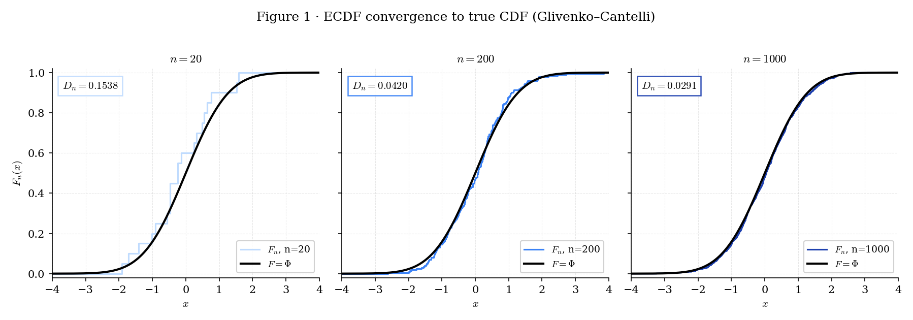
Figure 1. The empirical CDF of a standard-Normal sample at three sample sizes. At small the ECDF is visibly jagged; at large it is indistinguishable from the true CDF within plotting resolution.
Nonparametric statistics has two distinct meanings in the ML literature. The one Topic 29 cares about is distribution-free inference: the validity of a procedure does not depend on the form of . A bootstrap CI, a KS test, a Wilcoxon test, and a quantile CI built from order-statistic pairs are all distribution-free. The other meaning — “flexible modeling with infinite-dimensional parameters” — covers Bayesian nonparametrics (Dirichlet processes, Gaussian processes) and kernel methods; those are in formalml.
Distribution-freeness is what makes KS useful for real ML workflows: detecting distribution shift between training and deployment samples, validating that a model’s calibration stays the same across data slices, or checking that a simulator reproduces the empirical distribution of a sensor. None of those applications specify up front, so a t-test is the wrong tool.
Classical statistics assumes a parametric model; nonparametric statistics lets the data specify the model via the empirical distribution, and the order statistics are the lens through which we study that empirical distribution. §29.10’s forward-map spells out how Topics 30 (KDE), 31 (Bootstrap), and 32 (Empirical Processes) each sharpen one aspect of this sentence.
29.2 Order statistics: joint density
The order-statistic joint density has a clean closed form for continuous — one of the few places in statistics where a multivariate density has an elementary derivation via the change-of-variables formula.
For iid with continuous, the order statistics are the sorted sample, written with parenthesized indices:
The parentheses distinguish (the -th smallest value in the sample) from (the -th draw, in the order collected). When is continuous, ties occur with probability zero, so the inequalities are strict almost surely.
For iid with continuous CDF and density , the joint density of on the ordered simplex is
and zero outside that simplex. The marginal density of the -th order statistic is
(DAV2003 §2.1–§2.2.)
The joint density has a clean combinatorial reading: the factor counts the number of ways to assign unordered draws to ordered slots, and is the iid-joint density of the unordered sample. The marginal formula comes from integrating over the other coordinates and recognizing the binomial coefficient in the result — draws must fall below , must fall above, and one sits at .
For , the marginal density reduces to — the minimum’s density is the density at times the probability that the other draws are all above. For , the marginal is — the maximum’s density is times the probability the rest are all below. In both cases, as grows, the density concentrates near the lower or upper support endpoint respectively. The rate is governed by (upper tail) or (lower tail), which decays exponentially in away from the boundary — a topic fully developed at formalml extreme-value-theory.
The joint density of for comes from marginalizing Thm 1:
valid for . The combinatorial factor counts placements: below , one at , between, one at , above. §29.7 uses the special case to build distribution-free quantile CIs — pick so that .
For non-iid data (record values, concomitants, ranked-set sampling, progressive censoring) the joint density takes a different combinatorial form — the symmetry is broken. DAV2003 Chapters 5–6 develop the non-iid theory in full; Topic 29 restricts to iid throughout. The one use case outside iid order statistics that recurs in ML is censoring — survival analysis estimates from partially observed data — which we flag as an extension but do not develop.
Topic 16 §16 Thm 1 established that for any iid model, the order-statistic tuple is sufficient for : the conditional distribution of given does not depend on . The same result holds nonparametrically — for any , the order statistic captures every feature of the sample that influences. This is the structural justification for Track 8: the objects §29 develops are the raw features of every nonparametric procedure, because no statistic that respects the iid assumption can ever discard information in the order statistic. Independence notation (Topic 16 §16.9) carries forward: are not independent (ordering is the whole point), but for iid , the vector of ranks satisfies — a fact exploited by rank tests (forthcoming on formalml).
29.3 The uniform case and Rényi’s representation
The Uniform(0, 1) distribution is the reference case for order-statistic theory. Three facts make it special: the density is constant, so the marginal formula in Thm 1 collapses; the CDF is the identity, so the probability-integral transform connects it directly to the general- case; and the spacings (gaps between consecutive order statistics) have a surprisingly clean joint structure that Rényi exploited in 1953.
For iid , the -th order statistic has density
i.e. . This is Thm 1 specialized to on ; the Beta-density normalization follows from .
Corollary 1 (general ). If is the -th order statistic of an iid -sample and is continuous, then , since under the probability-integral transform, so sorting the -values gives the Uniform order statistics.
(DAV2003 §2.2.)
Corollary 1 is a universal statement: the Beta distribution governs regardless of . The OrderStatisticDensityBrowser below (Panel C) makes this visible — switching between Uniform, Exponential, and Normal changes the density of (Panels A and B), but the transformed statistic always sits on the same Beta curve.
Topic 7 §7.13 forward-promised this result as “coming soon”; Thm 2 + Cor 1 discharge it. The OrderStatisticDensityBrowser interactive lets the reader sweep from 1 to and watch the density shift from left to right across the support — a visual confirmation of the location for .
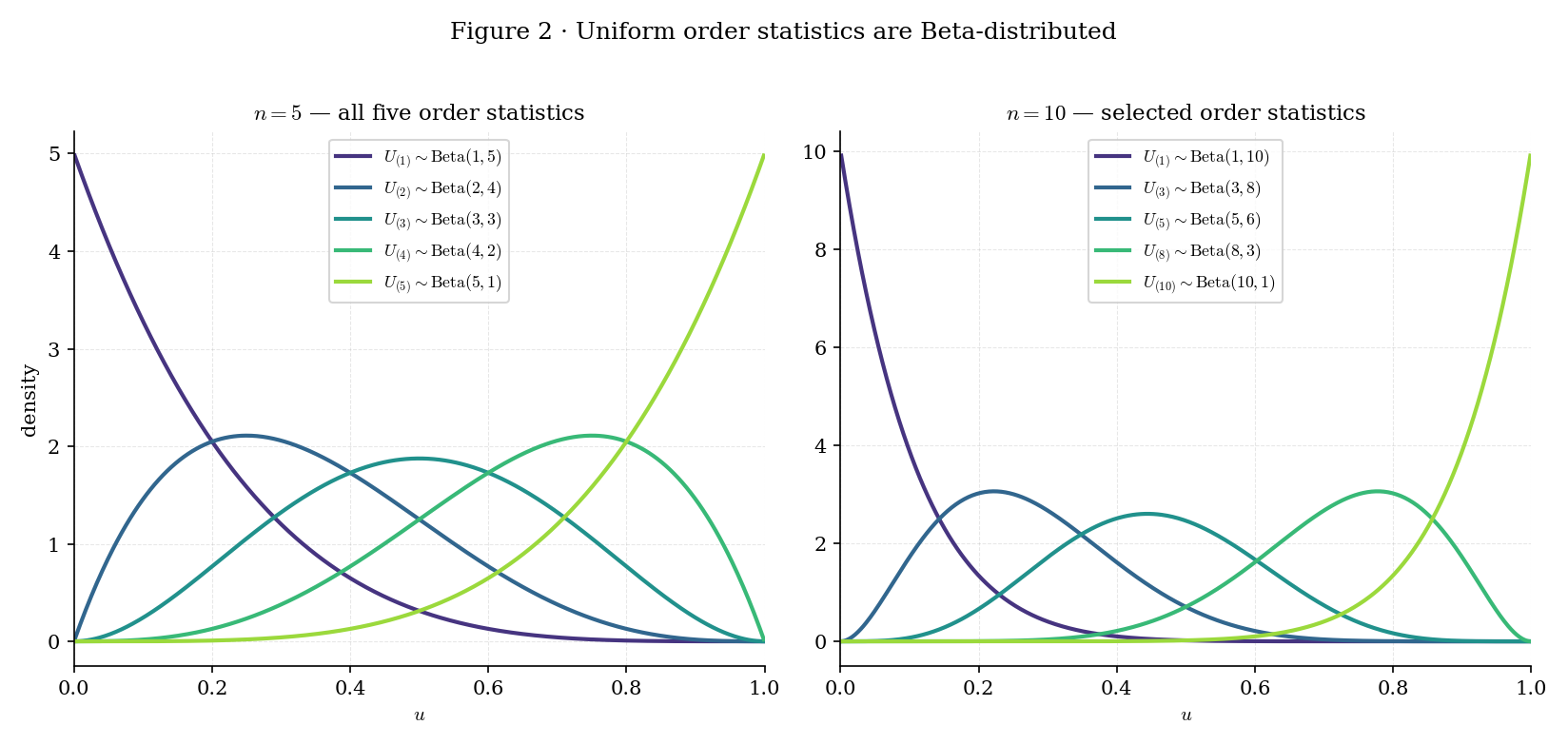
Figure 2. Uniform order-statistic densities at (left) and (right). Each curve is a Beta density with shape parameters — the reader can verify that the mean moves smoothly from the left endpoint toward the right endpoint as grows.
The uniform case has one further structural property that motivates a named theorem: the spacings of a Uniform(0, 1) sample — the gaps — have a clean distribution that Rényi (1953) discovered for the exponential case. Because Exp and Uniform are connected by (the inverse of the exponential CDF), the two stories are the same story. We state it for the exponential family where the algebra is prettiest.
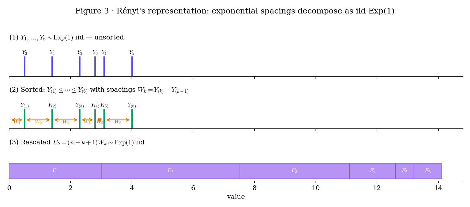
Figure 3. Rényi’s decomposition. Top: iid draws. Middle: sorted, with spacings between consecutive order statistics. Bottom: rescaled spacings , which Theorem 3 proves are iid .
Let be iid . Define the normalized spacings for (with ). Then the rescaled spacings are iid , and
where on the right-hand side are iid .
Proof 1 Proof of Thm 3 (Rényi's representation) [show]
The joint density of iid samples on the ordered simplex is
by Thm 1 specialized to the density on .
We change variables from to the spacings via (with ), so that . The Jacobian of this map is — the transformation matrix is lower-triangular with unit diagonal. The inverse image of the ordered simplex is the positive orthant .
The sum in the exponent rewrites as
where the swap of summation order counts how many times each appears in the sum of partial sums — namely times.
Substituting, the joint density of on the positive orthant is
This density factorizes across coordinates: are independent with . Note that , so the joint density is exactly the product of exponential densities with rates , confirming the normalization.
Defining rescales each coordinate by its rate, converting the coordinate into . So are iid . Finally,
— using the general order-statistic joint density (Thm 1), the Jacobian change-of-variables formula, and the factorization of the spacings density (REN1953; DAV2003 §2.5).
From Theorem 3,
where is the harmonic number. The minimum’s expectation is — the smallest of iid Exp(1) variables is itself Exp(), mean . The maximum’s expectation is — the largest of iid Exp(1) grows logarithmically. Both are lessons that recur in EVT (forthcoming on formalml): the maximum of iid Exp grows slowly, which is why the Gumbel distribution is the right asymptotic limit for Gumbel-domain tails.
The factor in Theorem 3 counts the “remaining” iid samples at step : among iid Exp(1) draws, the minimum is Exp(); conditional on the minimum, the second smallest is the minimum of the remaining — which by memorylessness is Exp(); and so on. The spacing structure is memorylessness in disguise. This is the exponential-family property that makes §29.6’s Bahadur residual have a clean form — the tail of the ECDF at quantile decomposes into iid contributions via the probability-integral transform onto Uniform, and then onto Exp via .
Rényi’s representation is the order-statistic reading of a Poisson-process fact: if we sprinkle iid -distributed inter-arrival times on , we get a Poisson process of rate . The sorted arrival times are , and the conditional distribution given is uniform order statistics on . Theorem 3 is a direct restatement of the inter-arrival independence in the forward direction. Point-process machinery (formalml point-processes, forthcoming) makes this connection structural.
Topic 16 §16.14 Ex 13 proved an unexpected consequence of Basu’s theorem: for iid , the ratio is independent of the maximum . The uniform-order-statistics structure Theorem 2 and Rényi’s representation exploit is the reason: once you change variables to the Uniform-order-statistics simplex, the joint density factorizes in ways that let Basu’s theorem detect independence cleanly. Basu in Topic 16 was an early hint of the uniform-order-statistics structure that §29.3 develops in full.
29.4 The sample quantile: Type 7
With order statistics in hand, we can define the sample quantile at level . The definition is less trivial than it looks: for with integer , the “obvious” answer is , but for in between — say with — there are many defensible choices. Hyndman and Fan (1996) catalogued nine conventions in use across statistical packages. Topic 29 adopts Type 7, the default in R, NumPy, and SciPy — matching a reader’s numpy environment is a pedagogical priority.
The population quantile at level is
For continuous strictly-increasing , in the usual inverse-function sense. The left-continuous-inverse definition handles atoms and flat regions of cleanly.
Let be the order statistics of an iid sample. The Type-7 sample quantile at level is
Equivalently: linearly interpolates between the two order statistics bracketing the position in the sorted sample. For , ; for , ; for with odd , , the sample median.
(HYN1996, default convention in R quantile(), NumPy quantile, SciPy scipy.stats.mstats.mquantiles.)
For the sample with : at , , so exactly. At , , so . At , , so . These match the numpy.quantile([1,2,3,4,5], q) defaults exactly — a sanity check that the Type-7 convention is what the reader’s tooling uses.
The nine Hyndman–Fan conventions differ in how they interpolate when is not at an integer order-statistic position. Type 1 (inverse-CDF) picks with no interpolation — it’s discontinuous in . Type 5 and Type 6 are older conventions still used in some engineering packages. Type 7 is the unique member of the family that (i) is a continuous piecewise-linear function of and (ii) hits the boundary exactly ( and ). Because R, NumPy, and SciPy all adopt Type 7 by default, a reader writing Python code to reproduce §29’s figures gets Type-7 numbers without setting a flag. Any other convention would introduce a silent discrepancy.
Exact sample quantiles require sorting the sample — and memory. In streaming or high-cardinality settings, approximate quantile sketches (Jain–Chlamtac 1985’s P² algorithm; Greenwald–Khanna 2001; Dunning’s t-digest 2021) trade small guaranteed error for bounded memory. These are widely used in ML production systems for real-time latency monitoring. Topic 29 does not develop them — streaming quantiles are an engineering sub-topic of its own. The relevant entry point is Dunning 2021 (t-digest) for practical use.
29.5 ECDF, Glivenko–Cantelli, DKW
Topic 10 §10.7 introduced the empirical CDF and proved it converges uniformly to almost surely — the Glivenko–Cantelli theorem. §29.5 sharpens that a.s. statement into a non-asymptotic bound via the Dvoretzky–Kiefer–Wolfowitz inequality, then converts DKW into a finite-sample confidence envelope that can be read off any realization of without knowing .
For iid with any CDF,
The supremum distance is the one-sample Kolmogorov–Smirnov statistic. Glivenko–Cantelli says almost surely. (Topic 10 §10.7 Thm 5; see there for the ε-net argument.)
Glivenko–Cantelli is qualitative — it says “eventually” is small — but does not tell us how small for any given . The Dvoretzky–Kiefer–Wolfowitz inequality provides a non-asymptotic exponential bound.
For iid and every ,
The constant is optimal (Massart 1990) when ; DVO1956 originally proved the bound with a larger, unspecified constant. Inverting the bound at confidence level gives a distribution-free finite-sample confidence envelope: the band with
contains uniformly in with probability .
Corollary 2 (the DKW envelope). With as above, regardless of . (DVO1956; MAS1990.)
DKW is a finite-sample strengthening of Glivenko–Cantelli that (i) holds for every , (ii) is distribution-free — does not appear in the bound — and (iii) has the optimal constant . It is the workhorse inequality behind every distribution-free uniform-deviation statement the rest of Track 8 uses. The envelope is a simultaneous confidence band for at every , not just a pointwise CI at a single .
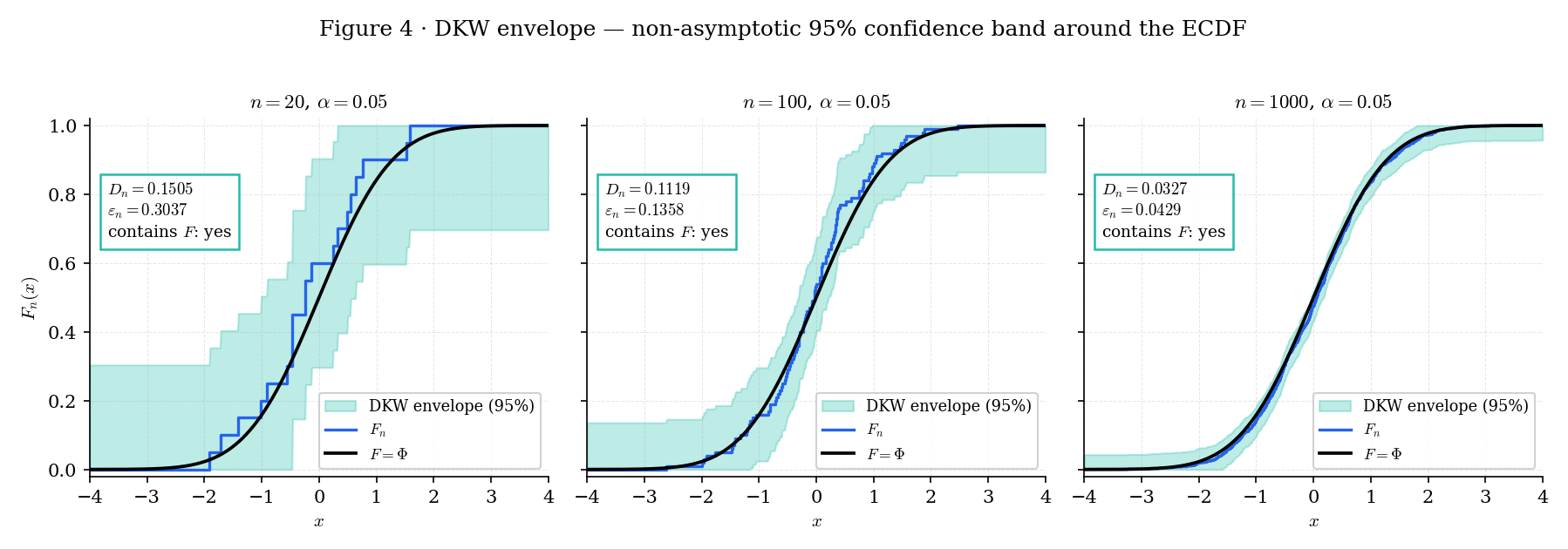
Figure 4. The DKW confidence envelope at . At the envelope is wide (±0.301) but already informative; at it narrows to ±0.043. The true CDF is contained by the envelope at every in each realization — this is guaranteed with probability by DKW, and the ECDFDKWBandExplorer below lets the reader empirically verify the coverage rate.
A common ML workflow: you suspect the distribution of a production feature has shifted since training. Collect training samples and production samples. Compute the ECDFs and and their sup-norm distance . The one-sample DKW envelopes give simultaneous confidence bands for the true train and production CDFs; if those bands overlap at every , no detectable shift. For the formal two-sample test — including the asymptotic null distribution — see §29.8 (with the two-sample variant a one-line extension to ksTwoSample in nonparametric.ts). Production systems run this test nightly to flag shift on each logged feature.
CLT says for each fixed — a pointwise asymptotic statement. DKW says is bounded non-asymptotically with probability — a uniform finite-sample statement. Both are useful: CLT gives the pointwise limiting distribution that §29.8 Thm 7 upgrades to uniform (via Donsker); DKW gives the uniform bound that does not require any asymptotic machinery. The Bahadur proof (§29.6) exploits both: CLT at the point plus a uniform-over-neighborhood fluctuation bound that DKW is the finite-sample analog of.
For at the median of , CLT gives asymptotic variance . DKW’s exponential rate at gives probability that the sup-norm gap is below , which matches the CLT tail probability to within constants. For deep in the tails where or , CLT gives much smaller pointwise variance than , so the DKW uniform bound is loose at tails — a property exploited by the tail-aware inequalities of Talagrand (Talagrand 1994) developed at formalml concentration-inequalities (forthcoming).
29.6 Bahadur representation and asymptotic normality
§29.6 is the centerpiece of Topic 29. Bahadur’s 1966 representation linearizes the sample quantile into an empirical-CDF term plus a small remainder — the same “score-function-like” decomposition that gives every classical estimator its asymptotic-normality corollary. The featured theorem + its corollary resolve the question “what is the limiting distribution of the sample median?” for essentially every distribution with positive density at its median, including heavy-tailed ones like the Cauchy where the usual variance-based CLT does not apply.
Let be iid with CDF . Fix and assume is differentiable at with and that is twice-differentiable in a neighborhood of with bounded second derivative. Let be the Type-7 sample quantile (Def 3). Then
where the remainder satisfies (Kiefer 1967 rate).
Corollary 1 (asymptotic normality). Under the same hypotheses,
(BAH1966; KIE1967; SER1980 §2.5; vdV2000 §21.)
The representation’s structure is the important part. The leading term is a linear functional of the ECDF evaluated at the true quantile — it is times a centered Bernoulli average with success probability and variance , which converges to a Normal by the CLT-for-indicators of §11 Thm 2. The remainder is smaller than — at the Kiefer rate — and is asymptotically negligible.
Corollary 1 falls out immediately: the leading term is Normal by CLT, the remainder is , and Slutsky’s lemma assembles them.
Proof 2 Proof of Thm 6 (Bahadur representation — featured) [show]
Throughout, write for the empirical CDF at a -scale neighborhood of . Define the centered empirical process . By the CLT applied to indicator variables (Topic 11 Thm 2), for each fixed ,
Step 1: Smoothness of near . By the second-derivative hypothesis and Taylor’s theorem,
for some between and . Since is bounded on a neighborhood of , the remainder is uniformly for with any fixed .
Step 2: The sample quantile equation. By the Type-7 definition, satisfies , which gives . Let denote the scaled quantile deviation. Substituting into ,
Using the Step-1 Taylor expansion,
Rearranging and multiplying by ,
Step 3: Approximate by . The empirical-process oscillation bound (Kiefer 1967 Thm 1; SER1980 §2.5 Thm A) states that for any fixed ,
Since (the sample quantile is root- consistent — which follows from the Step-2 equation plus the fact that is bounded in probability), we may restrict to on an event of probability tending to one, yielding
Step 4: Assemble the representation. Substituting into the Step-2 equation and recalling ,
Figure 5 renders here — the Monte Carlo decay of the median-absolute residual against the Kiefer envelope , verifying empirically what Step 4 proves analytically.
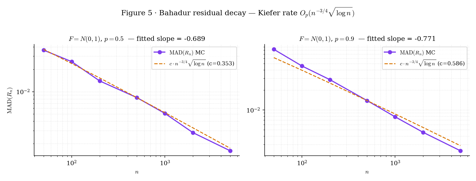
Figure 5. Empirical verification of the Kiefer rate. Left: ; right: . The slow-decaying factor means the empirical log-log slope is less negative than at moderate — the curves approach but don’t match the Kiefer envelope until . The QuantileAsymptoticsExplorer lets the reader verify this across distributions.
Step 5: Finalize. Dividing by and reading off ,
The remainder rate is sharp: Kiefer (1967) proved both the upper bound above and the matching lower bound .
— using Taylor’s theorem, the empirical-process oscillation bound (KIE1967 Thm 1), and CLT-for-indicators (Topic 11 Thm 2). Full details: BAH1966 for the original statement; KIE1967 for the sharp rate; SER1980 §2.5 and vdV2000 §21.2 for modern treatments.
The corollary’s asymptotic variance has a striking feature: it does not involve any moments of — only the value of the density at the population quantile. This is what makes the Bahadur representation the right tool for heavy-tailed data where moments may not exist. The QuantileAsymptoticsExplorer below makes this vivid via the Cauchy preset: Cauchy has no mean or variance, but its density at the median is , so the sample median’s limiting variance is — finite and small.
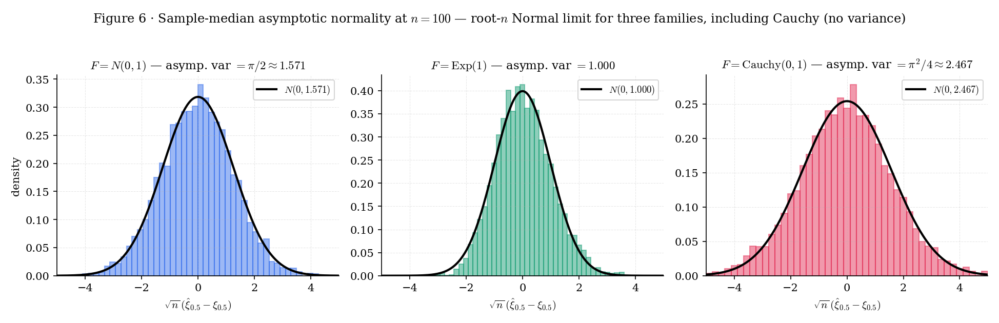
Figure 6. The Bahadur limit overlay for three distributions with very different moment behavior. Cauchy has no mean, no variance — but the sample median is still root- Normal, with limit variance finite because . The Bahadur representation is distribution-free in this sense: regularity lives at , not globally.
For at : , . Bahadur Cor 1 gives
The limiting standard error of the sample median is , compared to for the sample mean. The median is less efficient than the mean under exact Normal data by the factor — the asymptotic relative efficiency ARE(median, mean) = . Under heavier tails this ratio flips; see Ex 8.
For at : , . Bahadur Cor 1 gives
The limiting standard error is — slightly larger than the Normal case, but finite. The sample mean of Cauchy data is undefined asymptotically (the variance of is infinite; CLT does not apply), so the sample median is infinitely more efficient than the sample mean for Cauchy — ARE is . This is the money-shot example that motivates Bahadur: regularity is about the density at , not about moments.
The limit variance depends on — a nuisance parameter the reader typically does not know. Plug-in estimation requires estimating at . Topic 30 (Kernel Density Estimation) develops the general KDE machinery that provides consistent estimators with controlled bandwidth. The density-at-quantile problem is discharged at Topic 30 §30.7 Ex 9, which computes a Silverman-bandwidth KDE at the empirical quantile and plugs the result into Bahadur’s variance formula. Alternatively, the bootstrap (Topic 31: The Bootstrap) sidesteps this entirely by resampling the full empirical process — the plug-in variance is never computed directly.
The Bahadur representation is structurally identical to the Taylor-expansion-of-the-score-function argument that underpins MLE asymptotic normality (Topic 14 §14.6):
where the leading term is a mean-zero empirical average divided by a fixed constant, and the remainder is asymptotically negligible. Bahadur’s remainder rate is worse than MLE’s , but the functional form — “linearize into a known empirical average, bound the remainder, apply CLT” — is identical. Every Track 8 result reduces to a Bahadur-style linearization: KDE bandwidth asymptotics (Topic 30), bootstrap-CI validity (Topic 31: The Bootstrap), empirical-process functionals (Topic 32), and quantile-regression (forthcoming on formalml) all use this template.
Bahadur requires . At extreme — near 0 or 1 — the density may vanish ( or may be zero or undefined if the support is unbounded). In those regimes the sample quantile’s asymptotic distribution is not Normal at rate ; it is governed by the Fisher–Tippett–Gnedenko trichotomy (Gumbel, Fréchet, Weibull) at rate determined by the tail behavior of . Extreme-value theory is the subject of formalml extreme-value-theory (forthcoming); Topic 29 restricts to interior where Bahadur applies.
29.7 Distribution-free quantile confidence intervals
Bahadur Cor 1 gives an asymptotic CI for — but implementing it requires estimating . In some applications you want a CI whose validity does not require estimating any density. Order-statistic pairs provide exactly that: an exact (not asymptotic) finite-sample CI for whose coverage is a closed-form binomial probability, distribution-free.
For iid with continuous CDF , and , let be integers with . Then
regardless of . Choosing so that this binomial probability is yields a distribution-free exact -CI for . The canonical choice picks the largest with and the smallest with ; this gives a two-sided CI with exact coverage . (SER1980 §2.6.1.)
The key fact behind Theorem 7: the number of sample points is , since . So iff at least points fall below iff ; and iff at most points fall strictly below iff (using continuity to ignore ties). Combining gives the claim. Coverage is exactly the binomial tail probability — no asymptotics, no plug-in.
Because and are integers, coverage is a step function of : for the 95th-percentile CI at , the bounds shift discretely as crosses thresholds where the binomial tail probabilities change which integers are selected. The consequence: distribution-free quantile CIs over-cover at intermediate — the actual coverage is typically strictly greater than . Figure 7 makes this visible.
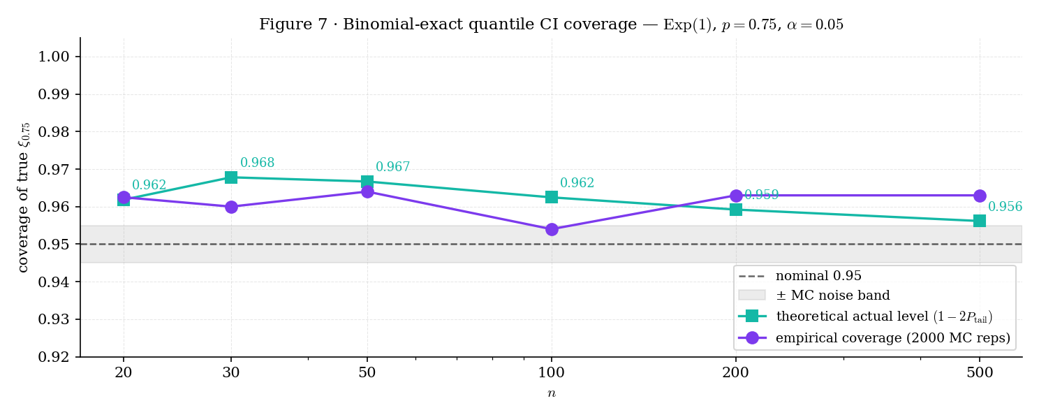
Figure 7. Empirical coverage of the 95% distribution-free CI for the 75th percentile of over 2,000 MC replicates. Coverage is a step function of : exact CIs over-cover at intermediate , tightening only when the binomial tail probabilities support a larger or smaller window. The 0.75 quantile-level was chosen over 0.95 because at with the binomial tail already exceeds from only the extreme pair, producing degenerate one-sided CIs that don’t illustrate the step structure pedagogically.
For , , : by symmetry of , the largest with is (since ), and symmetrically . The CI is , with exact coverage — slightly over-covering the nominal 0.95. This is the quantileCIOrderStatisticBounds(20, 0.5, 0.05) result pinned in the T29.15 test — , , actual level .
Production ML systems often set SLOs on latency percentiles — e.g., the 95th-percentile response time should be below 200ms. The distribution-free CI is a natural monitoring tool: collect request latencies in the past hour, compute at and . The resulting CI has guaranteed coverage without any assumption about the latency distribution — which matters because latency distributions are usually heavy-tailed (lognormal or Pareto-like) and asymptotic-Normal CIs based on are misleading in the tails. Conformal-prediction wrappers (forthcoming on formalml) generalize this construction to arbitrary prediction sets.
§29.7’s exact CI works specifically for quantiles — one of the few statistics where the coverage probability is binomial and closed-form. For a general statistic (mean, variance, regression coefficient), the same distribution-free spirit is captured by the bootstrap: resample from and use the empirical distribution of as the reference. Topic 31: The Bootstrap develops bootstrap-CIs in full (percentile, BCa, studentized), with Hall’s second-order accuracy result as the anchor. §19.10 Rem 20 punted bootstrap to Track 8; Topic 31 is where that promise lands. The order-statistic CI of §29.7 is the distribution-free CI “done in closed form” for quantiles specifically; the bootstrap is the general nonparametric CI machinery for every other statistic.
29.8 The Kolmogorov–Smirnov test
§29.5 Thm 4 restated Glivenko–Cantelli’s almost surely, and Thm 5 gave the non-asymptotic DKW bound. §29.8 completes the picture: the asymptotic distribution of is the Kolmogorov distribution, and this yields the one-sample Kolmogorov–Smirnov goodness-of-fit test — testing whether an iid sample was drawn from a specified continuous CDF .
Let be iid from a continuous CDF and let . Then
where is the Kolmogorov distribution with CDF
The asymptotic null distribution is distribution-free: it does not depend on . The partial proof below assumes Donsker’s theorem (proved at Topic 32 §32.5) and derives the Kolmogorov limit as a consequence. (KOL1933; SMI1948; BIL1999 §14.)
Proof 3 Proof of Thm 8 (Kolmogorov-distribution limit, partial) [show]
The proof has three ingredients: (i) the probability-integral transform reduces the general- case to ; (ii) Donsker’s theorem — taken as given here, proved at Topic 32 — gives a distributional limit for the normalized empirical process; (iii) the continuous mapping theorem extracts the sup-norm distribution from that limit.
Ingredient (i): reduce to uniform. Define . Since is continuous, . The empirical CDF of at level equals the empirical CDF of at :
Substituting gives , so
which is the KS statistic for the uniform case. Henceforth assume .
Ingredient (ii): Donsker’s theorem (proved at Topic 32 §32.5). Define the uniform empirical process for . Donsker’s theorem (BIL1999 §16) states that converges in distribution in the space (with the Skorokhod topology) to a standard Brownian bridge — a centered Gaussian process on with covariance and boundary conditions . Topic 32 develops the full empirical-process machinery — including the Skorokhod topology, tightness arguments, and finite-dimensional convergence — and proves Donsker as its centerpiece. Here we take it as given.
Ingredient (iii): continuous mapping. The sup-norm functional defined by is continuous — indeed, 1-Lipschitz with respect to the uniform metric. By the continuous mapping theorem (Topic 9 §9.5),
The Kolmogorov formula. The distribution of is classical (BIL1999 §14 Thm 14.4):
This is derived from the reflection principle applied to Brownian motion and conditioning on ; we quote the formula rather than re-deriving it, since the full derivation uses the Brownian-motion technology developed at formalml stochastic-processes. Combining with Ingredient (iii) gives the claimed limit.
(assuming Donsker — proved at Topic 32 — and the sup-norm-of-Brownian-bridge distribution — quoted from BIL1999 §14.4.)
The KS statistic with the asymptotic Kolmogorov null distribution gives the one-sample KS test. Critical values are standard: , , , all divided by for the un-scaled statistic.
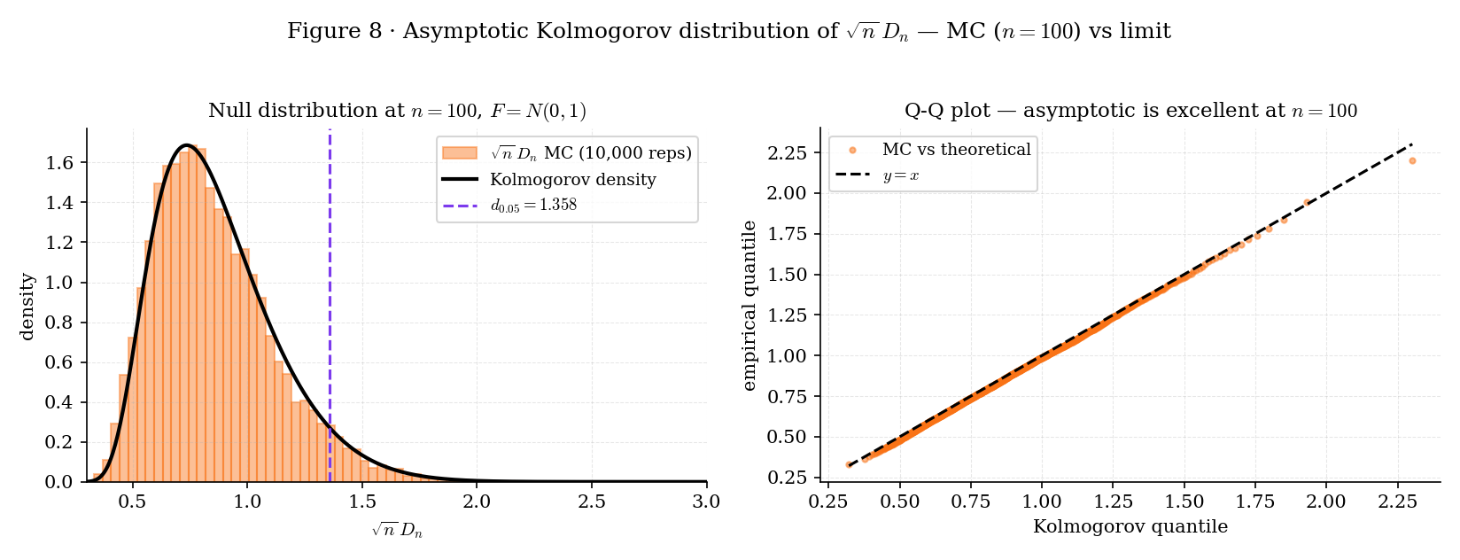
Figure 8. Empirical validation of the Kolmogorov asymptotic at . Left: MC histogram of under with the Kolmogorov density overlay — nearly exact match. Right: Q-Q plot against the Kolmogorov quantile function — points lie on the diagonal. The asymptotic is reliable for ; for smaller , the Smirnov finite-sample formula (SMI1948) is more accurate.
Train a classifier on last month’s data, deploy this month. Pull 500 prediction confidences from last month’s validation set and 500 from this month’s live traffic. Run KS on each feature (or on the confidence scores themselves) against the training ECDF. Large relative to triggers retraining. This is the most common KS application in production ML — and it is distribution-free in exactly the sense §29.1 Rem 1 emphasizes: no assumption about the shape of the confidence distribution.
A common calibration check for probabilistic classifiers: the probability-integral transform (PIT) values should be Uniform(0, 1) if the predictive distribution is well-calibrated. Running KS on the PIT values against Uniform is a standard calibration test. KS detects systematic miscalibration (e.g., the classifier is overconfident and PIT is concentrated near 0 and 1) without assuming any specific miscalibration structure. Gneiting–Raftery 2007 develops the full calibration theory; the KS test is the entry-level distribution-free version.
For , the asymptotic Kolmogorov CDF is not a great approximation to the finite-sample null distribution of . Smirnov (SMI1948) gives a finite-sample formula based on the combinatorial reflection principle; modern implementations (scipy.stats.kstest, R ks.test) use Smirnov’s formula for small and the Kolmogorov asymptotic for (or thereabouts — the exact crossover depends on the implementation). For ML production workflows where is typically , the asymptotic is always sufficient. The nonparametric.ts module ships the asymptotic-only ksPValue for component usage; wrapping SciPy’s exact formula is standard for notebook-side work.
29.9 ML bridges: ranks, conformal prediction, quantile regression
Three themes recur in the ML literature that use the nonparametric machinery of §§29.2–29.8 as substrate. Topic 29 states their structural connection and forward-points to dedicated development.
The rank transform replaces each by its rank in the sorted sample — a discrete analog of the probability-integral transform. For iid continuous , the rank vector is uniform on the symmetric group, independent of the order statistic, and governs the null distribution of Wilcoxon’s signed-rank test, Mann–Whitney’s U test, and Kruskal–Wallis’s multi-sample test. These rank tests are permutation-based nonparametric alternatives to t-tests / F-tests / ANOVA, valid without any distributional assumption. They are the standard tool when the data are ordinal, or when the distributional shape is unknown and the user does not want to risk KS’s loss of power to narrow-band alternatives. Full development: formalml rank-tests (forthcoming).
Conformal prediction (Vovk–Gammerman–Shafer 2005; Shafer–Vovk 2008) is a modern machine-learning tool that builds distribution-free prediction intervals around any black-box predictor . The construction: given a calibration set and a non-conformity score (e.g., ), the -conformal prediction interval for a new is
where is the sample quantile of the calibration non-conformity scores. The coverage guarantee is distribution-free — it follows from exchangeability alone, with no parametric assumption on . §29.7’s order-statistic CI is the distribution-free CI for the population quantile; conformal prediction applies the same exchangeability argument to the quantile of a learned score function. Full development: formalml conformal-prediction (forthcoming).
Topic 29’s sample quantile estimates the scalar intercept of a distribution with no covariates. Quantile regression (Koenker–Bassett 1978; Koenker 2005) extends this to the covariate-conditional case: estimate , the -quantile of the conditional distribution. The estimator minimizes the check loss averaged over the sample, a convex loss tied directly to the population quantile. Topic 15 §15.9 already named check-loss regression as the natural-forward-pointer target; Topic 29 discharges the scalar case via §29.4/§29.6, and formalml quantile-regression (forthcoming) handles the conditional extension. L-statistics and trimmed means (SER1980 §8) are a sibling topic — linear functionals of the order-statistics vector — covered in §31 (bootstrap asymptotics) and formalml.
29.10 Track 8 forward-map and spine
Track 8 has three topics after this one:
- Topic 30 — Kernel Density Estimation (KDE). The density in Bahadur’s denominator is estimated non-parametrically via kernel smoothing of the ECDF. KDE is “what happens when you differentiate using a smooth weighting function.” The Silverman rule-of-thumb bandwidth, cross-validation bandwidth selection, and higher-order kernels all sit there.
- Topic 31 — The Bootstrap (published). The bootstrap replaces the unknown with (the ECDF) and resamples with replacement. Every bootstrap statement is a pushforward of Topic 29’s ECDF-convergence results through a functional. Hall’s second-order accuracy for BCa is the anchor result.
- Topic 32 — Empirical Processes & Uniform Convergence (track closer, now published). The functional view: for function classes . DKW, Bahadur, and the Kolmogorov distribution are all consequences of Donsker’s theorem — the empirical process converges to the Gaussian Brownian-bridge process in for Donsker classes. Topic 32 proves Donsker; Topic 29 used it once (§29.8 Thm 7).
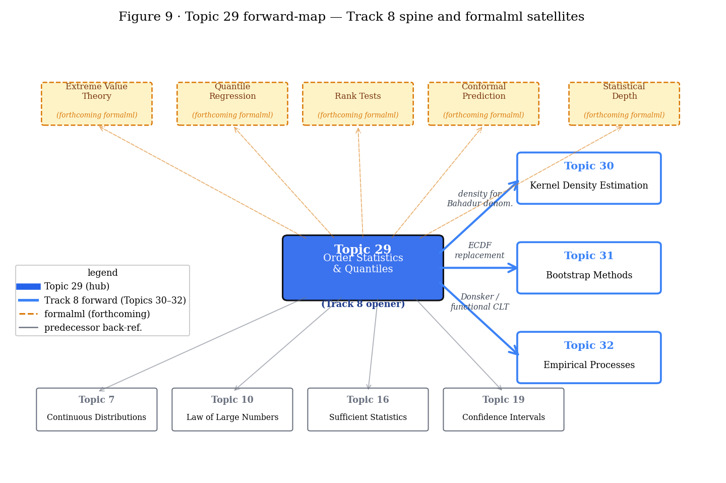
Figure 9. The Track 8 spine, as seen from its opener. Topic 29 → 30, 31, 32 build the full nonparametric-and-empirical-process toolkit; the five formalml satellites develop domain-specific applications (extremes, quantile regression, rank tests, conformal, depth).
Topic 29’s Bahadur asymptotics cover for interior , where . When (or 0), the density vanishes and Bahadur fails. The correct asymptotic theory — the Fisher–Tippett–Gnedenko trichotomy (Gumbel, Fréchet, Weibull) — lives at formalml extreme-value-theory (forthcoming). The maximum , properly centered and rescaled, converges in distribution to one of three limit types depending on the tail behavior of . EVT is essential for risk management (financial tail losses), reliability engineering (component failure times), and LLM-latency worst-case bounds.
Koenker–Bassett 1978 quantile regression extends §29.4/§29.6’s scalar-intercept case to the conditional case . Check-loss minimization yields estimators with Bahadur-style asymptotic normality — the linearization survives, but the influence function now involves the conditional density at each covariate value. Full development: formalml quantile-regression (forthcoming).
Wilcoxon signed-rank, Mann–Whitney U, and Kruskal–Wallis are the three classical rank-based nonparametric alternatives to the t-test, two-sample t-test, and one-way ANOVA respectively. The permutation-distribution machinery they depend on is orthogonal to Topic 29’s Bahadur asymptotics — the null distribution comes from rank uniformity, not from empirical-process limits. A proper treatment requires its own chapter. Full development: formalml rank-tests (forthcoming). §18.10 Rem 25 previewed this as Track 8 territory.
Conformal prediction (VOV2005; SHA2008) wraps any black-box predictor with distribution-free prediction intervals using exchangeability and quantile machinery. §29.7’s order-statistic CI is the distribution-free CI for the population quantile; conformal prediction is the distribution-free CI for a learned score function’s quantile. The two are the same idea at different levels of generality. Full development: formalml conformal-prediction (forthcoming).
Topic 29 is scalar throughout — one-dimensional . For multivariate , there is no canonical ordering, so the univariate order-statistic / quantile machinery does not apply directly. Statistical depth functions — Tukey depth, Mahalanobis depth, halfspace depth, zonoid depth — generalize the quantile function to multivariate settings. Full development: formalml statistical-depth (forthcoming). The univariate case is embedded naturally: Tukey depth in 1D reduces to , recovering §29.4’s via the level set of depth.
Track 8’s organizing thesis, stated at the top of §29.1 and worth repeating here: classical statistics assumes a parametric model; nonparametric statistics lets the data specify the model via the empirical distribution, and the order statistics are the lens through which we study that empirical distribution. Everything that follows — KDE’s smoothing of into a density, bootstrap’s pushforward of through a functional, empirical processes’ view of as a random function — reads that thesis at a different zoom level.
References
- Bahadur, R. R. (1966). A Note on Quantiles in Large Samples. Annals of Mathematical Statistics, 37(3), 577–580.
- Kiefer, J. (1967). On Bahadur’s Representation of Sample Quantiles. Annals of Mathematical Statistics, 38(5), 1323–1342.
- Rényi, A. (1953). On the Theory of Order Statistics. Acta Mathematica Academiae Scientiarum Hungaricae, 4(3–4), 191–231.
- Dvoretzky, A., Kiefer, J., & Wolfowitz, J. (1956). Asymptotic Minimax Character of the Sample Distribution Function and of the Classical Multinomial Estimator. Annals of Mathematical Statistics, 27(3), 642–669.
- Massart, P. (1990). The Tight Constant in the Dvoretzky–Kiefer–Wolfowitz Inequality. Annals of Probability, 18(3), 1269–1283.
- Smirnov, N. V. (1948). Table for Estimating the Goodness of Fit of Empirical Distributions. Annals of Mathematical Statistics, 19(2), 279–281.
- Kolmogorov, A. N. (1933). Sulla determinazione empirica di una legge di distribuzione. Giornale dell’Istituto Italiano degli Attuari, 4, 83–91. (Historical Italian journal; no stable URL.)
- David, H. A., & Nagaraja, H. N. (2003). Order Statistics (3rd ed.). Wiley.
- Hyndman, R. J., & Fan, Y. (1996). Sample Quantiles in Statistical Packages. The American Statistician, 50(4), 361–365.
- Serfling, R. J. (1980). Approximation Theorems of Mathematical Statistics. Wiley.
- Lehmann, E. L., & Casella, G. (1998). Theory of Point Estimation (2nd ed.). Springer.
- van der Vaart, A. W. (2000). Asymptotic Statistics. Cambridge University Press.
- Billingsley, P. (1999). Convergence of Probability Measures (2nd ed.). Wiley.