One long dependent sample. The autocovariance function determines a stationary series up to second order, and it can be read in time or in frequency: the Wold decomposition writes every stationary series as a moving average of its own prediction errors, and Herglotz's theorem turns the same autocovariance into a spectral density. ARMA models are the finite-parameter family dense in both views — causality and invertibility are root conditions, and the spectrum is a ratio of distances to those roots. Nine full proofs, featuring Wold by orthogonal projection; Yule–Walker, Durbin–Levinson, the inconsistent periodogram and its smoothed repair, and GARCH as the observation-driven answer to Topic 34's hidden regimes.
Three datasets an ML practitioner meets every week: the daily validation error of a forecasting model across two years of backtests, the 5,000 draws of an MCMC chain, a sensor log sampled once a second. Each is one long sample whose observations lean on their neighbors. Almost every confidence interval we built in Tracks 4–6 divided a standard deviation by n, and that division quietly assumed the n observations were independent. This topic asks what survives when they aren’t.
The answer runs through one object. For a series whose statistical behavior doesn’t drift, the covariance between two observations depends only on how far apart they are, and that function of the gap, the autocovariance functionγ(h), determines everything second-order. We can read it in time (prediction, the Wold decomposition, ARMA models) or in frequency (a spectral density). Both readings pay off in ML: the long-run variance behind an MCMC chain’s effective sample size is the spectral density at frequency zero, and a stationary Gaussian-process kernel is a spectrum.
Example 1 A naive confidence interval on autocorrelated data
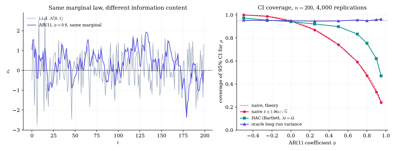
Simulate an autoregression with unit marginal variance, Xt=ϕXt−1+1−ϕ2Zt with Zt i.i.d. N(0,1), the parameterization of Topic 26’s Example 8. Every Xt is N(0,1), whatever ϕ is; only the dependence between neighbors changes. Take n=200 observations and form the textbook 95% interval for the mean, xˉ±1.96s/n, where xˉ is the sample mean and s the sample standard deviation. Over 4,000 replications the interval covers the true mean μ=0:
0.946 of the time at ϕ=0 (independent data: the interval works);
0.331 of the time at ϕ=0.9, against the theoretical value 2Φ(1.96(1−ϕ)/(1+ϕ))−1=0.347, where Φ is the standard Normal CDF;
0.9995 of the time at ϕ=−0.5: negative dependence makes neighbors cancel, so the naive interval over-covers.
An interval built with the true long-run variance (Theorem 2) covers 0.958 at ϕ=0.9. The standard econometric fix, a Newey–West interval with bandwidth M=4 (Remark 6), recovers only to 0.621. At ϕ=0.9 the variance of Xˉ is about 19/n, not 1/n, so 200 observations carry the information of about 10.5 independent ones.
Figure 1. Same marginal distribution, different information. An interval that ignores autocorrelation covers the truth a third of the time when φ = 0.9.
Example 2 Backtested model errors
Two forecasting models are compared on two years of daily losses. The loss difference dt=ℓt(A)−ℓt(B) is positively autocorrelated, because both models miss the same regime shifts. If the differences are as persistent as Example 1’s ϕ=0.9 series, the naive standard error s/n of their mean is too small by a factor σLR2/γ(0)=19≈4.36, where σLR2 is Theorem 2’s long-run variance. A “significant” improvement can be pure dependence; Remark 21 says how to estimate the right standard error.
Remark 1 Notation
A time series is a sequence of random variables {Xt:t∈Z} indexed by the integers; we call it the process. The data are one realization x1,…,xn of n consecutive values. We write E[X] for the expectation (the center of mass of X‘s distribution), Var(X)=E[(X−EX)2] for the variance, and Cov(X,Y)=E[(X−EX)(Y−EY)] for the covariance. Time is discrete: t counts steps.
Remark 2 Two coordinates for one object
Everything second-order lives in γ(h). Sections 35.2–35.6 read it in time: averages, prediction, Wold, ARMA, estimation. Sections 35.7–35.8 read it in frequency: the spectral density, the periodogram, smoothing. Section 35.9 shows what γ cannot see: a GARCH series has the autocovariance of white noise, yet predictable volatility.
35.2 Stationarity and the autocovariance function
To learn from a single realization, the process must repeat itself statistically: days 1–100 must say something about days 101–200. Stationarity is that assumption, in two strengths.
Definition 1 Strict stationarity
A process {Xt} is strictly stationary if shifting time leaves every finite-dimensional distribution unchanged: for every k≥1, all times t1,…,tk and every shift h, the vector (Xt1+h,…,Xtk+h) has the same joint distribution as (Xt1,…,Xtk).
Definition 2 Weak stationarity; autocovariance and autocorrelation functions
A process {Xt} is weakly stationary if EXt2<∞, the mean EXt=μ does not depend on t, and the covariance between two observations depends only on how far apart they are:
Cov(Xt+h,Xt)=γ(h)for all t,h∈Z.
The function γ is the autocovariance function (ACVF) and ρ(h)=γ(h)/γ(0) is the autocorrelation function (ACF). Directly from the definition, γ(0)=Var(Xt)≥0, γ(−h)=γ(h), and ∣γ(h)∣≤γ(0) by the Cauchy–Schwarz inequality.
Definition 3 White noise
A process {εt} is white noise with variance σ2, written εt∼WN(0,σ2), if Eεt=0, Var(εt)=σ2, and Cov(εs,εt)=0 for s=t. The stronger assumption that the εt are independent and identically distributed is written IID(0,σ2). White noise is uncorrelated, not necessarily independent; GARCH (§35.9) will be white noise whose squares are correlated.
Which functions can be autocovariances? Not every even function: for any coefficients a1,…,an and times t1,…,tn,
i,j∑aiγ(ti−tj)aj=Var(i∑aiXti)≥0,
so γ must be nonnegative definite. That turns out to be the whole story.
Theorem 1 Characterization of autocovariance functions (stated; BRO1991 Thm 1.5.1)
A function γ:Z→R is the autocovariance function of a weakly stationary series if and only if it is even and nonnegative definite: ∑i,j=1naiγ(ti−tj)aj≥0 for all n, all real a1,…,an, and all integers t1,…,tn.
Necessity is the variance identity above; sufficiency builds a Gaussian process with covariance γ by Kolmogorov’s extension theorem.
Example 3 Four ACFs
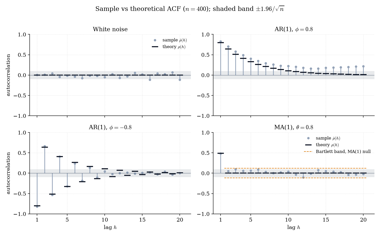
Simulate n=400 observations from four processes and compare the sample ACF (Remark 5) with the theory.
White noise:ρ(h)=0 for every h=0. The sample autocorrelations scatter inside the band ±1.96/n=±0.098, the approximate 95% range when the true value is zero (Theorem 9).
AR(1), ϕ=±0.8: the autoregression Xt=ϕXt−1+εt has ρ(h)=ϕ∣h∣, alternating in sign when ϕ<0 (Example 5 derives it). At ϕ=0.8, ρ(5)=0.3277, but the sample value is 0.4053: sample autocorrelations wander from the truth in runs (Remark 5).
MA(1), θ=0.8: the moving average Xt=εt+θεt−1 has ρ(1)=θ/(1+θ2)=0.4878 (sample 0.4808) and ρ(h)=0 for h≥2: two observations more than one step apart share no shock. Under this MA(1) the correct band beyond lag 1 is wider than the white-noise band, ±0.1185, because Bartlett’s formula (Theorem 9) adds the variance contributed by ρ(1).
Figure 2. Four autocorrelation functions. Sample autocorrelations wander in runs, so a single lag outside the band is weak evidence.
Now the theorem behind Example 1: the variance of a mean of dependent observations picks up every pairwise covariance.
Theorem 2 Long-run variance
Let {Xt} be weakly stationary with mean μ and autocovariance γ satisfying ∑h∈Z∣γ(h)∣<∞, and let Xˉn=n−1∑t=1nXt. Then
nVar(Xˉn)=∣h∣<n∑(1−n∣h∣)γ(h)⟶σLR2:=h∈Z∑γ(h).
Consequently E(Xˉn−μ)2→0 and XˉnPμ.
Proof 1 Proof of Thm 2 (Long-run variance) [show][hide]
Expand the variance of the sum as a double sum of covariances:
Let n→∞: the first term vanishes, so the limsup is at most ∑∣h∣>K∣γ(h)∣, and letting K→∞ makes that tail 0. Hence nVar(Xˉn)→σLR2. Since EXˉn=μ, E(Xˉn−μ)2=Var(Xˉn)=(σLR2+o(1))/n→0, and Chebyshev’s inequality gives P(∣Xˉn−μ∣>ε)≤Var(Xˉn)/ε2→0.
■ — using the triangle inequality, tails of absolutely convergent series, and Chebyshev’s inequality (Topic 10).
◼
The first display is exact for every n, and its weights 1−∣h∣/n are Fejér’s; they reappear in the mean of the periodogram (Proof 8). The corollary is an ergodic weak law: the sample mean is consistent, at rate σLR/n rather than σ/n.
Example 4 MCMC effective sample size, recovered
Topic 26’s AR(1) chain Xt+1=0.9Xt+0.19Zt is stationary with γ(0)=1 and γ(h)=0.9∣h∣. Theorem 2’s long-run variance is
h∈Z∑γ(h)=1+2h≥1∑0.9h=1−0.91+0.9=19,
which is exactly the integrated autocorrelation time τ of Topic 26 Def 7. A chain of 5,000 draws is worth Neff=5000/19≈263 independent draws, matching Topic 26 Example 8’s Geyer estimate.
Remark 3 The ergodic WLLN extends Topic 10's uncorrelated case
Topic 10 §10.3 proved the weak law for uncorrelated sequences, which is the special case γ(h)=0 for h=0, where σLR2=γ(0). Theorem 2 needs only summable correlations, and consistency alone needs only γ(h)→0, since the Cesàro average n−1∑∣h∣<n(1−∣h∣/n)γ(h) then vanishes. Summability buys the 1/n rate.
Remark 4 Weak versus strict; Gaussian processes
Strict stationarity plus a finite second moment implies weak. The converse fails in general, except for a Gaussian process, whose finite-dimensional laws are fixed by means and covariances (Topic 8). Most theorems here need only weak stationarity; Theorem 15 (GARCH) works with strict.
Remark 5 Why the sample ACVF divides by n
The sample autocovariance is
γ^(h)=n1t=1∑n−h(xt+h−xˉ)(xt−xˉ),0≤h<n,
and ρ^(h)=γ^(h)/γ^(0) is the sample ACF. Dividing by n rather than n−h biases γ^(h) toward zero at large lags, but makes the sample covariance matrix Γ^n=[γ^(i−j)] nonnegative definite (it equals n−1TT⊤ for a matrix T of shifted copies of the demeaned data), which Yule–Walker needs (Remark 15). Sample autocorrelations at nearby lags are strongly correlated (Theorem 9), which is why Example 3’s AR(1) sample ACF stays above the theory for a run of lags.
Remark 6 HAC: estimating the long-run variance
Example 1’s oracle interval used the true σLR2. In practice we estimate it, and the plug-in ∑∣h∣<nγ^(h) is inconsistent — it equals 2π times the periodogram at frequency zero, which §35.8 shows never settles down. The Newey–West estimator (NEW1987) truncates and down-weights the sample autocovariances:
σ^LR2=γ^(0)+2h=1∑M(1−M+1h)γ^(h).
With the common rule M=⌊4(n/100)2/9⌋=4 at n=200, it lifts Example 1’s coverage from 0.331 to only 0.621 at ϕ=0.9: the truncation lag M is a bandwidth, too small for a series this persistent (Remark 21). This is the HAC covariance used in GMM with dependent data: formalML: generalized-method-of-moments .
35.3 Prediction as projection and the Wold decomposition
Random variables with finite variance form a vector space. Give it the inner product ⟨U,V⟩=E[UV] (the covariance, for zero-mean variables) and it becomes the Hilbert space L2 ( formalCalculus: hilbert-spaces ). Length is standard deviation, orthogonality is uncorrelatedness, and the mean squared error of a prediction is the squared distance between the prediction and the target.
So predicting Xn+1 linearly from the past means finding the closest point to Xn+1 in the subspace spanned by the past — an orthogonal projection — and the prediction error is the part of Xn+1 orthogonal to everything we have seen. Taken to the infinite past, that picture is the Wold decomposition.
Definition 4 Linear process
A linear process is a series of the form
Xt=μ+j=−∞∑∞ψjεt−j,εt∼WN(0,σ2),j∑∣ψj∣<∞.
It is causal if ψj=0 for j<0, so that Xt depends only on present and past shocks. The infinite sum converges in L2 and almost surely (Topic 9), and because the covariance is continuous in L2 we may compute it term by term: by bilinearity and the uncorrelatedness of white noise, γ(h)=σ2∑jψjψj+∣h∣.
Example 5 MA(q) and AR(1) as linear processes
A moving average of order q, Xt=εt+θ1εt−1+⋯+θqεt−q, is a linear process with ψ0=1, ψj=θj for 1≤j≤q, and ψj=0 otherwise. Since ψjψj+∣h∣=0 for ∣h∣>q, its autocovariance vanishes beyond lag q.
An AR(1)Xt=ϕXt−1+εt with ∣ϕ∣<1 becomes a linear process by substituting the equation into itself k times:
Xt=j=0∑k−1ϕjεt−j+ϕkXt−k.
The remainder has E(ϕkXt−k)2=ϕ2kγ(0)→0, so in L2, Xt=∑j≥0ϕjεt−j: ψj=ϕj. Definition 4’s formula then gives
γ(h)=σ2j≥0∑ϕjϕj+∣h∣=1−ϕ2σ2ϕ∣h∣,
which discharges Example 3’s promise that ρ(h)=ϕ∣h∣. For ϕ=0.9 and σ2=1, γ(0)=1/0.19=5.263158.
Definition 5 Best linear predictor; innovations; deterministic series
Let {Xt} be zero-mean and weakly stationary. Write Hn=sp{Xs:s≤n} for the closed linear span of the infinite past (all L2 limits of finite linear combinations). The best linear predictor of Xn+1 is the projection X^n+1=PHnXn+1, the innovation is εn+1=Xn+1−X^n+1, and the one-step mean squared error is σ2=Eεn+12, which does not depend on n by stationarity. The series is deterministic if σ2=0 (the past predicts the future perfectly) and purely nondeterministic if ⋂nHn={0} (the remote past carries no information).
With only finitely many observations, PnXn+1 denotes the projection onto sp{X1,…,Xn}, with mean squared error vn.
The finite-past projection reduces to linear algebra, and the stationarity of γ makes that algebra recursive.
Theorem 3 Prediction equations and Durbin–Levinson
Let {Xt} be zero-mean weakly stationary with γ(0)>0 and γ(h)→0 as h→∞. Write Γn=[γ(i−j)]i,j=1n and γn=(γ(1),…,γ(n))⊤.
(i) The best linear predictor of Xn+1 from X1,…,Xn is PnXn+1=∑j=1nϕnjXn+1−j, where ϕn=(ϕn1,…,ϕnn)⊤ is the unique solution of Γnϕn=γn, and its mean squared error is vn=γ(0)−ϕn⊤γn.
Proof 2 Proof of Thm 3 (Prediction equations and Durbin–Levinson) [show][hide]
(i) Let M=sp{X1,…,Xn}, a finite-dimensional, hence closed, subspace of L2. By the projection theorem (formalCalculus: Hilbert spaces), PnXn+1 is the unique X^∈M with Xn+1−X^⊥Xk for k=1,…,n. Write X^=∑jϕnjXn+1−j and impose orthogonality to Xn+1−i:
which is Γnϕn=γn. Under γ(0)>0 and γ(h)→0, Γn is nonsingular for every n (BRO1991 Prop. 5.1.1), so the coefficients are unique. Because the error is orthogonal to X^∈M, vn=E[(Xn+1−X^)Xn+1]=γ(0)−∑jϕnjγ(j).
(ii) Stationarity makes prediction time-reversible: the equations for predicting X1 from X2,…,Xn have the same Toeplitz matrix Γn−1 and right-hand side as those for predicting Xn+1 from the same variables in reverse order. So with K=sp{X2,…,Xn},
and both errors have mean square vn−1. The space M splits orthogonally as K⊕sp{U} with U=X1−PKX1, so projecting onto each piece,
PnXn+1=PKXn+1+aU,a=EU2E[Xn+1U].
The denominator is vn−1. The numerator is E[Xn+1X1]−∑jϕn−1,jE[Xn+1X1+j]=γ(n)−∑jϕn−1,jγ(n−j), so a is the claimed ϕnn. Expanding aU and collecting the coefficient of Xn+1−j (which appears in U as X1+(n−j)) gives ϕnj=ϕn−1,j−ϕnnϕn−1,n−j, and the coefficient of X1 is ϕnn. Finally, Xn+1−PnXn+1=(Xn+1−PKXn+1)−aU with aU the projection of the first term onto sp{U}, so by Pythagoras
vn=vn−1−a2EU2=vn−1−ϕnn2vn−1.
■ — using the projection theorem, the orthogonal decomposition M=K⊕sp{U}, and the time-reversal symmetry of γ (LEV1947, DUR1960).
◼
Solving Γnϕn=γn directly costs O(n3); the recursion builds every predictor up to order n in O(n2) and produces the partial autocorrelations ϕnn of §35.5 for free.
Example 6 Forecasting an AR(1), and how fast forecasts fade
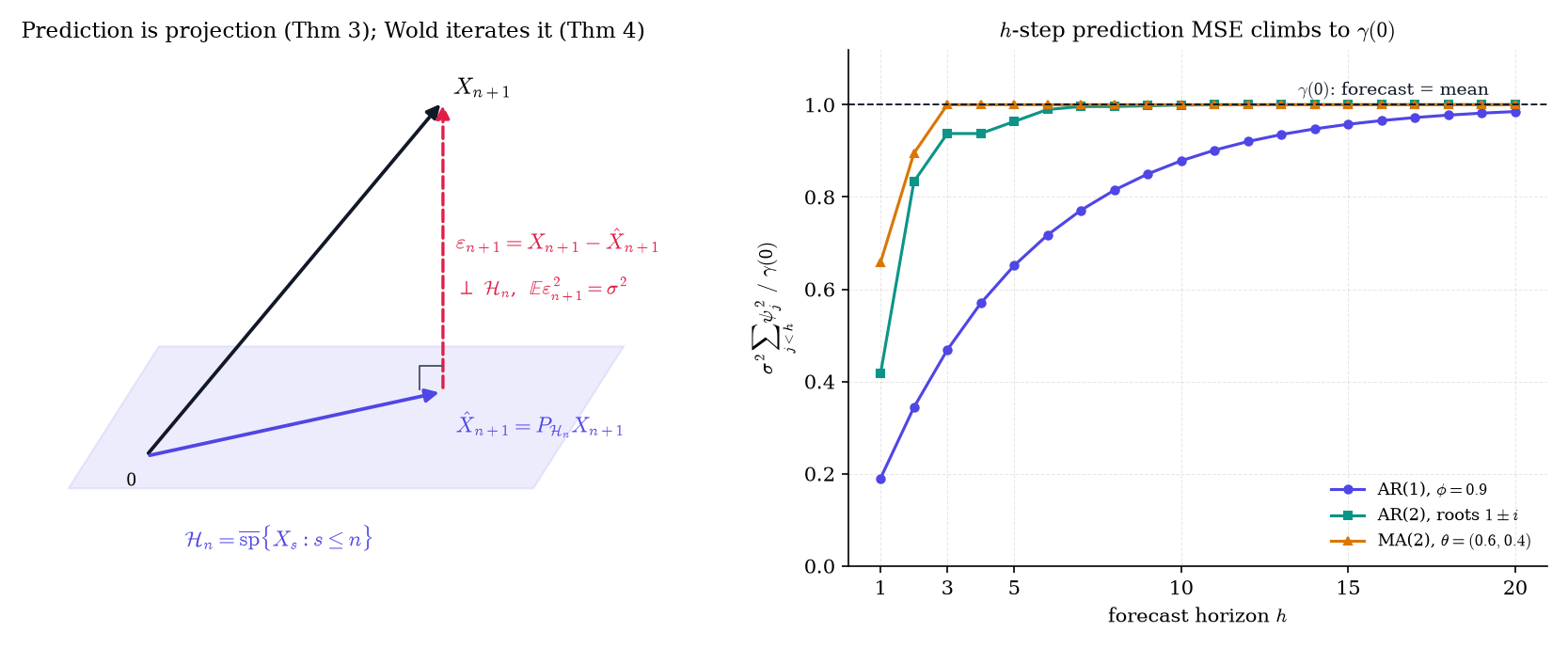
For a causal linear process in its own innovations, the h-step forecast drops the shocks not yet seen, so its mean squared error is σ2∑j<hψj2. For the AR(1), PnXn+h=ϕhXn and the MSE is γ(0)(1−ϕ2h). As a fraction of the variance γ(0):
AR(1), ϕ=0.9:0.19 at h=1, so the past explains 81% of the variance (0.81); 0.651322 at h=5.
AR(2) with roots 1±i:0.416667 at h=1, 0.963542 at h=5.
MA(2), θ=(0.6,0.4):0.657895 at h=1, and exactly 1 from h=3 on. An MA(q) is unpredictable beyond q steps.
Now the featured theorem: push the projection to the infinite past and ask what is left once every innovation is projected out.
Theorem 4 Wold decomposition
Let {Xt} be zero-mean weakly stationary, Ht=sp{Xs:s≤t}, and suppose the one-step prediction error σ2=E(Xt−PHt−1Xt)2 is positive. Then
Xt=j=0∑∞ψjεt−j+Vt,
where (i) εt=Xt−PHt−1Xt is WN(0,σ2) and εt∈Ht; (ii) ψ0=1, ψj=E[Xtεt−j]/σ2 does not depend on t, and ∑jψj2<∞; (iii) E[εsVt]=0 for all s,t; (iv) Vt∈H−∞=⋂sHs; (v) {Vt} is deterministic: Vt lies in the closed span of {Vs:s<t}.
Proof 3 Proof of Thm 4 (Wold decomposition) [show][hide]
Step 1 (the shift is unitary). Define U on finite combinations by U∑iaiXti=∑iaiXti+1. Inner products depend only on lag differences, so U preserves them; it extends to a unitary map of H=sp{Xt:t∈Z} onto itself with UHt−1=Ht. Projections commute with it: PHtXt+1=UPHt−1Xt, hence εt+1=Uεt.
Step 2 (innovations are white noise). By the projection theorem εt⊥Ht−1. For s<t, εs∈Hs⊆Ht−1, so E[εtεs]=0. By Step 1, Eεt2=Eε02=σ2, and Eεt=0. This is (i).
Step 3 (the moving-average part). The family {εt−j/σ}j≥0 is orthonormal in Ht. Projecting Xt onto its closed span Mt gives the Fourier expansion
which converges in L2 because Bessel’s inequality gives σ2∑jψj2≤EXt2. Unitarity makes ψj=⟨Xt,εt−j⟩/σ2 independent of t, and ψ0=E[(PHt−1Xt+εt)εt]/σ2=1 because εt⊥Ht−1. This is (ii).
Step 4 (the remainder is orthogonal to every innovation). Set Vt=Xt−PMtXt, so Vt⊥εs for s≤t. For s>t, Xt∈Hs−1 and εs⊥Hs−1, while each εt−j in the expansion also lies in Hs−1; so Vt⊥εs as well. This is (iii).
Step 5 (the remainder lives in the remote past). Since Xt=PHt−1Xt+εt, we have Ht=Ht−1⊕sp{εt}. Now Vt∈Ht and Vt⊥εt, so Vt∈Ht−1. Repeating with Ht−1=Ht−2⊕sp{εt−1} and Vt⊥εt−1 gives Vt∈Ht−2, and by induction Vt∈Ht−k for every k. This is (iv).
Step 6 (the remainder is deterministic). For s≤t−1, Xs=∑jψjεs−j+Vs with the two parts orthogonal, so Ht−1=Mt−1⊕Vt−1, where Vt−1=sp{Vs:s≤t−1}. By (iv), Vt∈Ht−1, and by (iii) it is orthogonal to Mt−1, so Vt∈Vt−1: its own past predicts it with zero error. This is (v).
■ — using the projection theorem, Bessel’s inequality and L2 convergence of orthonormal expansions, and the unitary shift on H (WOL1938; BRO1991 Thm 5.7.1).
◼
So what does Wold buy us? A purely nondeterministic series (Vt=0) is exactly a causal MA(∞) in its own innovations, and those innovations are its one-step forecast errors. Every forecasting model is a choice of how to approximate the infinite sequence ψj with finitely many parameters; ARMA is the next section’s answer.
Figure 3. Prediction is projection. The innovation is the part of tomorrow orthogonal to everything we have seen, and forecast error climbs to the full variance as the horizon grows.
Drag the forecast origin and stretch the horizon: the band widens to ±1.96γ(0) as the Wold weights run out, and for an AR(p) every Durbin–Levinson bar beyond p is exactly zero.
Let Xt=Acos(λt)+Bsin(λt), where A and B are uncorrelated with mean 0 and common variance σA2, and λ∈(0,π) is a fixed frequency. The angle-addition formula gives γ(h)=σA2cos(λh), so the series is stationary. It is also exactly predictable: the trigonometric identity cos(λt)=2cosλcos(λ(t−1))−cos(λ(t−2)), and the same for sines, gives
Xt=2cos(λ)Xt−1−Xt−2
with no error term, so σ2=0 and Wold’s Vt is the whole series. Its spectrum (§35.7) is two point masses at ±λ, a spectral distribution without a density.
Remark 7 Wold is about linear prediction only
The innovations are uncorrelated, not independent. A GARCH series (§35.9) is white noise, so its Wold representation is trivial (ψ0=1, all other ψj=0), yet its squared returns are predictable. Linear prediction is blind to volatility; that blindness is §35.9’s subject.
Remark 8 The prediction-error decomposition, and Topic 36
For a Gaussian series the joint density of x1,…,xn factors into one-step predictions:
where x^t is the best linear predictor of xt from x1,…,xt−1 and vt−1 its mean squared error. The exact likelihood is a product of one-step prediction errors. Theorem 3 computes the x^t and vt in O(n2) operations; Topic 36 computes them in O(n) with the Kalman filter, after writing an ARMA model in state-space form.
Remark 9 Gaussian series: linear is optimal
If {Xt} is a Gaussian process, PnXn+1=E[Xn+1∣X1,…,Xn]: the best linear predictor is the best predictor of any kind. This is the conditional multivariate Normal formula of Topic 8 §8.4, with Γn as the conditioning covariance block. Outside the Gaussian case the conditional mean can beat every linear predictor.
35.4 ARMA models: causality and invertibility
Wold says every purely nondeterministic series is an MA(∞). An infinite sequence of weights is too many parameters, so we want ψj generated by finitely many numbers. Ratios of polynomials do exactly that, and the theory of the family lives in where those polynomials have their roots.
Definition 6 ARMA(p, q)
Write B for the backshift operator, BXt=Xt−1, so BkXt=Xt−k. Define the AR polynomial and MA polynomial
ϕ(z)=1−ϕ1z−⋯−ϕpzp,θ(z)=1+θ1z+⋯+θqzq.
A zero-mean series {Xt} is an ARMA(p, q) process if it is stationary and
ϕ(B)Xt=θ(B)εt,εt∼WN(0,σ2),
that is, Xt−ϕ1Xt−1−⋯−ϕpXt−p=εt+θ1εt−1+⋯+θqεt−q. We require that ϕ and θ have no common zeros: a shared factor cancels from both sides and the model is over-parameterized. A series with mean μ is ARMA if Xt−μ is.
Definition 7 Causal; invertible
An ARMA process is causal if Xt=∑j≥0ψjεt−j with ∑j∣ψj∣<∞: the present is built from present and past shocks only. It is invertible if εt=∑j≥0πjXt−j with ∑j∣πj∣<∞: the shocks can be recovered from present and past observations. The ψj are the MA(∞) weights and the πj the AR(∞) weights.
Causality is what a forecaster needs; invertibility is what an estimator needs, since the likelihood is built from shocks recovered from the data. Both are statements about the unit circle.
Theorem 5 Causality: AR roots outside the unit circle
Let ϕ(B)Xt=θ(B)εt with ε∼WN(0,σ2), where ϕ and θ have no common zeros. A causal stationary solution Xt=∑j≥0ψjεt−j with ∑j∣ψj∣<∞ exists if and only if ϕ(z)=0 for all complex ∣z∣≤1. In that case the solution is unique and ∑jψjzj=θ(z)/ϕ(z) for ∣z∣≤1.
Proof 4 Proof of Thm 5 (Causality) [show][hide]
(⇐) Factor ϕ(z)=∏k=1p(1−z/rk) over its roots, all with ∣rk∣>1. Each factor inverts as a geometric series,
(1−rkz)−1=j=0∑∞rk−jzj,j∑∣rk∣−j<∞,
absolutely convergent on ∣z∣≤1. The Cauchy product of finitely many absolutely summable sequences is absolutely summable ( formalCalculus: power-taylor-series ), so 1/ϕ(z)=∑jξjzj with ∑j∣ξj∣<∞, and so is ψ(z)=ξ(z)θ(z). Define Xt=∑jψjεt−j, a causal linear process (Def 4). Applying absolutely summable filters to a stationary sequence is legitimate, and composing two such filters multiplies their power series (absolute convergence lets us rearrange the double sum). Hence
ϕ(B)Xt=ϕ(B)ξ(B)θ(B)εt=θ(B)εt,
because ϕ(z)ξ(z)=1. For uniqueness, let Y be any stationary solution and apply ξ(B) to ϕ(B)Yt=θ(B)εt: Yt=ξ(B)θ(B)εt=Xt.
(⇒) Suppose Xt=ψ(B)εt with ∑∣ψj∣<∞. Then θ(B)εt=ϕ(B)Xt=η(B)εt with η(z)=ϕ(z)ψ(z)=∑jηjzj, absolutely summable. Take the covariance of both sides with εt−j: white noise kills every term but one, leaving σ2θj=σ2ηj for every j≥0 (with θj=0 for j>q). So ϕ(z)ψ(z)=θ(z) on ∣z∣≤1, where both sides converge absolutely. If ϕ(z0)=0 for some ∣z0∣≤1, then θ(z0)=ϕ(z0)ψ(z0)=0, a common zero — contradicting the hypothesis.
■ — using geometric series, absolute convergence of Cauchy products, and uncorrelatedness of white noise.
◼
No complex analysis was needed — only that ∑j∣r∣−j converges exactly when ∣r∣>1. That single inequality is why “outside the unit circle” is the boundary.
Theorem 6 Invertibility: MA roots outside the unit circle
In the setting of Theorem 5, εt=∑j≥0πjXt−j with ∑j∣πj∣<∞ if and only if θ(z)=0 for all ∣z∣≤1, and then ∑jπjzj=ϕ(z)/θ(z) for ∣z∣≤1.
Proof 5 Proof of Thm 6 (Invertibility) [show][hide]
This is Proof 4 with the roles of ϕ and θ exchanged. (⇐) Factoring θ over its roots, all outside the closed disk, gives 1/θ(z)=∑jζjzj with ∑∣ζj∣<∞. Applying ζ(B) to ϕ(B)Xt=θ(B)εt,
ζ(B)ϕ(B)Xt=ζ(B)θ(B)εt=εt,
so π(z)=ζ(z)ϕ(z) works and is absolutely summable. (⇒) If εt=π(B)Xt, apply π(B) to the ARMA equation and use that absolutely summable filters commute:
π(B)θ(B)εt=π(B)ϕ(B)Xt=ϕ(B)π(B)Xt=ϕ(B)εt.
Matching coefficients by covariance with εt−j, exactly as in Proof 4, gives π(z)θ(z)=ϕ(z) on ∣z∣≤1. A zero of θ in the closed disk would be a zero of ϕ too, a common zero.
■ — using the argument of Proof 4 with ϕ and θ exchanged.
◼
Example 8 Three AR(1)s, one innovation sequence
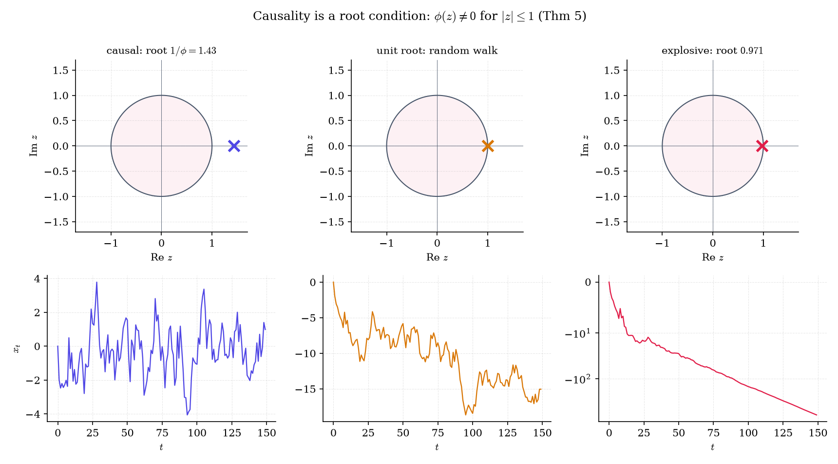
Drive three AR(1) recursions Xt=ϕXt−1+εt with the same 150 shocks, starting from X0=0. The polynomial 1−ϕz has the single root 1/ϕ.
ϕ=0.7: root 1/0.7=1.43, outside the circle. Shocks are forgotten geometrically and the path hovers near zero (final value 0.984).
ϕ=1: root exactly on the circle, a unit root. The recursion is a random walk, Xt=X0+ε1+⋯+εt, whose variance grows linearly in t; it wanders to −15.0 by t=150.
ϕ=1.03: root 0.971, inside the circle. Shocks are amplified and the path explodes to −614.
For ∣ϕ∣>1 a stationary solution still exists, Xt=−∑j≥1ϕ−jεt+j, but it is built from future shocks: non-causal and useless for forecasting.
Figure 4. Causality is a root condition. Outside the unit circle the series forgets its shocks; on it, it wanders; inside, it explodes.
Example 9 AR(2): complex roots, and a unit root in disguise
Take ϕ=(1,−0.5), so ϕ(z)=1−z+0.5z2. Its roots are 1±i, of modulus 2=1.41421>1: the model is causal. Complex roots at angle ±π/4 make the solution of the recursion a damped cosine, so the ACF oscillates with period 2π/(π/4)=8 steps while decaying like ∣r∣−h=2−h/2 (Figure 5, top).
Now take ϕ=(1.2,−0.2). Both coefficients look harmless, but ϕ(z)=1−1.2z+0.2z2=(1−z)(1−0.2z) has roots 1 and 5. The root at 1 sits on the circle, so there is no causal stationary solution. The first difference Xt−Xt−1 is a causal AR(1) with coefficient 0.2: this is an ARIMA(1, 1, 0) (Remark 12).
Example 10 ψ and π weights of an ARMA(1, 1)
For ϕ(z)=1−0.7z and θ(z)=1+0.4z, match coefficients of zj in ϕ(z)ψ(z)=θ(z): ψ0=1, ψ1−0.7ψ0=0.4, and ψj−0.7ψj−1=0 for j≥2. So ψj=(ϕ+θ)ϕj−1=1.1⋅0.7j−1 for j≥1:
ψ0,…,ψ5=1,1.1,0.77,0.539,0.3773,0.26411.
Matching coefficients in θ(z)π(z)=ϕ(z) instead gives π0=1, π1+0.4=−0.7, and πj+0.4πj−1=0 for j≥2:
π0,…,π5=1,−1.1,0.44,−0.176,0.0704,−0.02816.
The ψj decay at the rate of the AR root (0.7=1/1.43), the πj at the rate of the MA root (0.4=1/2.5).
Drag the AR roots (×) and MA roots (○) around the unit circle and watch causality, invertibility, the ACF and PACF, and the spectrum respond. The spectrum panel previews §35.7: hover over it to draw the distance from e−iω to every root; the spectrum is a ratio of those distances.
Preset:
ARMA(2, 0) · drag a root, or Tab to it and use the arrow keys (Shift for bigger steps)
Causal and invertible: every root lies outside the unit circle.
Remark 10 Roots, the companion matrix, and stability
An AR(p) is a first-order recursion in disguise. Stack Yt=(Xt,Xt−1,…,Xt−p+1)⊤; then Yt=ΦYt−1+et, where the companion matrixΦ has (ϕ1,…,ϕp) as its first row and ones on the subdiagonal, and et=(εt,0,…,0)⊤. Its eigenvalues are the reciprocals of the roots of ϕ(z), so causality says the spectral radius of Φ is below 1 — the stability condition of linear dynamical systems ( formalCalculus: stability-dynamics , formalCalculus: eigenvalues-eigenvectors ). This first-order vector form is exactly the state-space representation Topic 36 starts from.
Remark 11 Non-invertible MA models are not identifiable from γ
An MA(1) with parameters (θ,σ2) and one with (1/θ,θ2σ2) have the same autocovariance: both give γ(0)=σ2(1+θ2) and γ(1)=σ2θ. Reflecting any MA root r inside the circle to 1/rˉ, and rescaling σ2, leaves γ unchanged, so we always report the invertible twin. The explorer’s Flip button performs exactly this reflection, and the ACF panel doesn’t move.
Remark 12 ARIMA and unit roots
If ϕ(z)=(1−z)dϕ∗(z) with ϕ∗ causal, then the d-th difference (1−B)dXt is a causal ARMA, and Xt is an ARIMA(p, d, q) process. Differencing removes the unit root. Deciding whetherd=1 is harder: the Dickey–Fuller test (DIC1979) has nonstandard asymptotics, since in a random walk the least-squares ϕ^ converges at rate n, not n, to a non-Gaussian limit. We leave unit-root testing aside; see formalML: random-walks .
35.5 Identification: ACF and PACF
Which ARMA(p, q) should we fit? An MA(q) has an ACF that is exactly zero beyond lag q (Example 5). For autoregressions a second function cuts off: the correlation between Xt and Xt−hafter the intermediate observations have had their say.
Definition 8 Partial autocorrelation
The partial autocorrelation function (PACF) of a stationary series is α(1)=ρ(1) and, for h≥2, α(h)=ϕhh, the last coefficient of the best linear predictor of Xh+1 from Xh,…,X1 (Theorem 3). Equivalently, α(h) is the correlation between Xh+1 and X1 after both have been regressed on X2,…,Xh — it is the coefficient a of Proof 2.
Durbin–Levinson computes every α(h) as a by-product, and for autoregressions it delivers a cutoff.
Theorem 7 The AR(p) PACF cuts off after lag p
If {Xt} is a causal AR(p), ϕ(B)Xt=εt with ϕp=0, then α(p)=ϕp and α(h)=0 for every h>p.
Proof 6 Proof of Thm 7 (PACF cutoff) [show][hide]
Fix h≥p and consider the candidate predictor X^=∑j=1pϕjXh+1−j, which lies in sp{X1,…,Xh} because h+1−p≥1. Its error is Xh+1−X^=εh+1. By causality (Theorem 5) each Xs with s≤h is an L2 limit of combinations of εr, r≤s≤h, and εh+1 is uncorrelated with all of them. Hence
E[(Xh+1−X^)Xs]=E[εh+1Xs]=0,s=1,…,h,
so X^ satisfies the orthogonality conditions that characterize PhXh+1 (Theorem 3(i)). Because those conditions have a unique solution, ϕhj=ϕj for j≤p and ϕhj=0 for p<j≤h. Reading off the last coefficient: α(h)=ϕhh equals ϕp when h=p and 0 when h>p.
■ — using causality (Theorem 5), the projection characterization and uniqueness in Theorem 3(i), and Definition 8.
◼
The dual statement needs no new proof: an MA(q)‘s ACF is zero beyond lag q (Definition 4 with ψj=0 for j>q). An ARMA with both p,q≥1 has neither cutoff, because its ψj and πj are both infinite sequences.
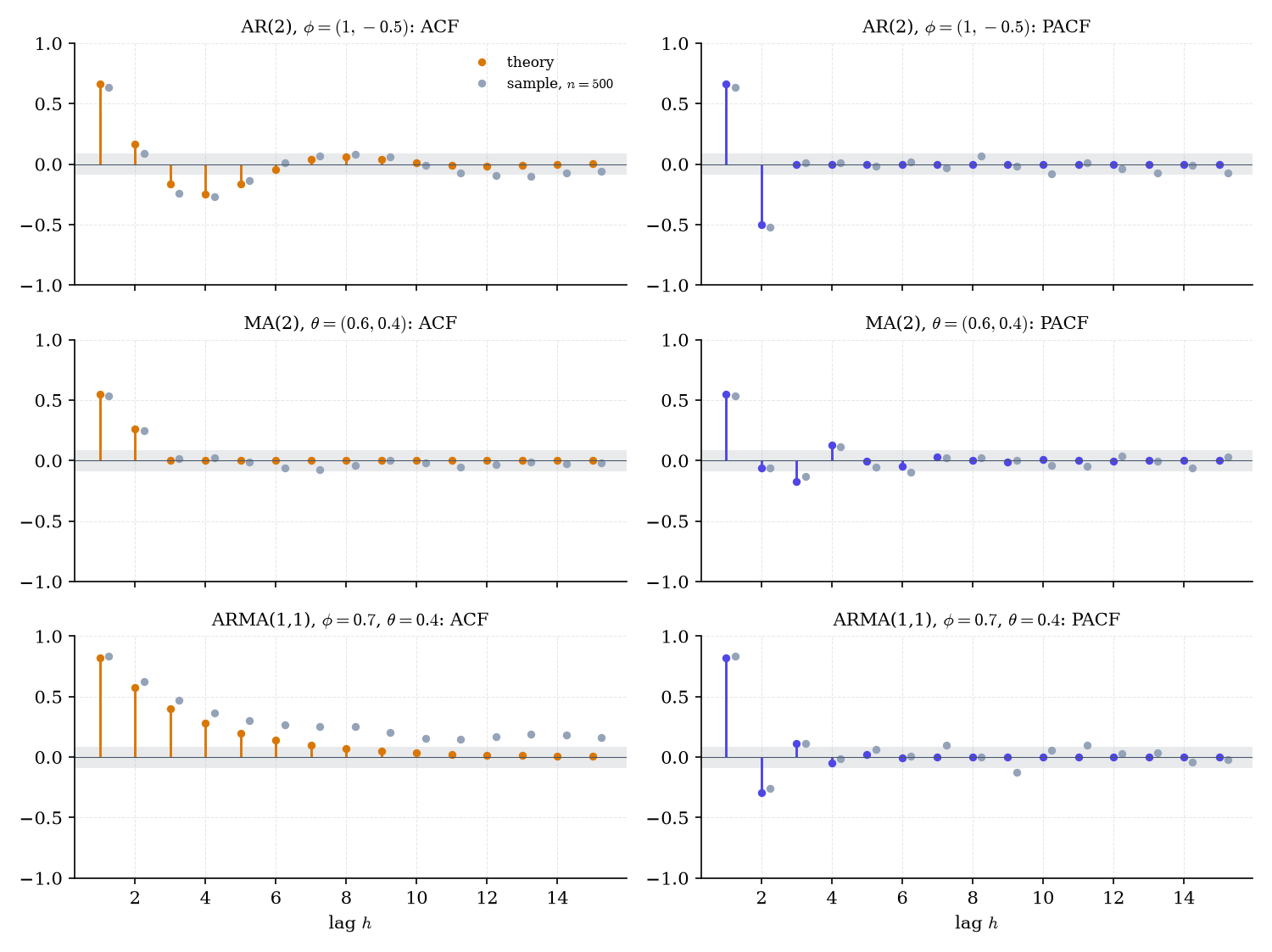
Example 11 The identification grid
Theory and a simulated sample of n=500 for three models:
AR(2), ϕ=(1,−0.5):ρ(1)=α(1)=2/3=0.666667, α(2)=−0.5=ϕ2, and α(3)=0, as Theorem 7 requires. The ACF is a damped cosine; ρ(3)=−0.166667.
MA(2), θ=(0.6,0.4):ρ(1)=0.84/1.52=0.552632, ρ(2)=0.4/1.52=0.263158, and ρ(3)=0. The PACF tails off instead: −0.0608 and −0.1744 at lags 2 and 3.
ARMA(1, 1), ϕ=0.7, θ=0.4:ρ(1)=α(1)=0.818605 and α(2)=−0.294314; both functions tail off geometrically.
Figure 5. The identification table, drawn. An AR(p) PACF stops after lag p; an MA(q) ACF stops after lag q; an ARMA tails off in both.
Remark 13 The identification table and the Box–Jenkins loop
Model
ACF
PACF
AR(p)
tails off
cuts off after lag p
MA(q)
cuts off after lag q
tails off
ARMA(p, q)
tails off
tails off
Box and Jenkins (BOX2015) built a loop around this table: identify an order from the sample ACF and PACF, estimate, check the residuals, repeat. Modern practice identifies with the information criteria of §35.6 and keeps the table as a sanity check.
35.6 Estimation and order selection
Three estimators cover almost all practice. Yule–Walker replaces γ by γ^ in Theorem 3’s prediction equations: solve Γ^pϕ^=γ^p, set σ^2=γ^(0)−ϕ^⊤γ^p, and compute both by Durbin–Levinson — a method-of-moments estimator. Conditional least squares (CSS) regresses xt on its lags as in Topic 21; with MA terms it minimizes ∑tet2 over residuals computed recursively, et=xt−∑jϕjxt−j−∑jθjet−j, starting from et=0 (“conditional” on that start). Gaussian maximum likelihood maximizes Remark 8’s exact likelihood (Topic 14).
Example 12 Yule's sunspot autoregression, 1927
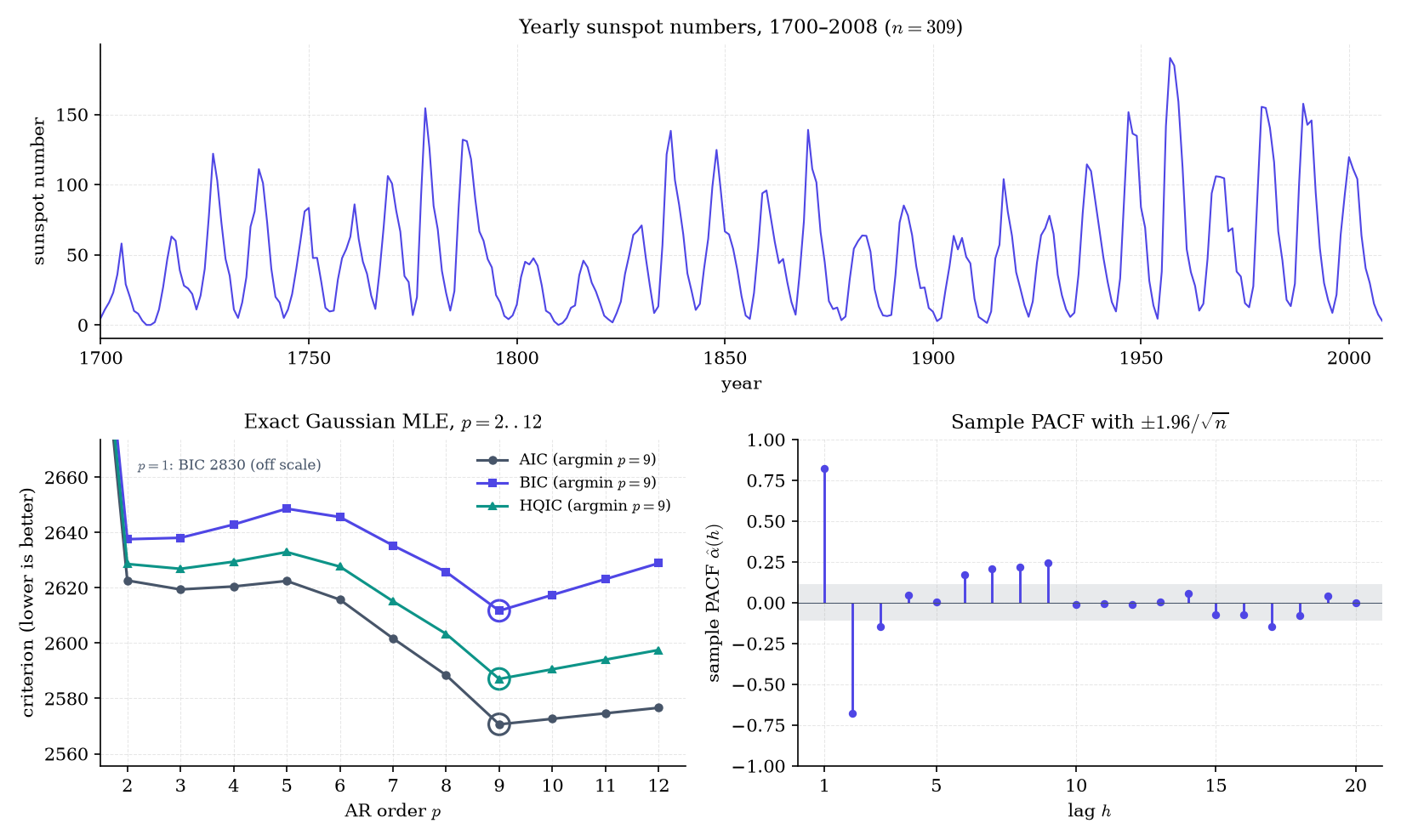
Yearly sunspot numbers from 1700 to 2008 (n=309, the SIL1981 series) rise and fall with the roughly eleven-year solar cycle. Fitting an AR(2) by Yule–Walker gives
ϕ^=(1.375227,−0.676694),σ^2=289.373.
The roots of ϕ^(z) are complex with modulus 1.21564, at an angle giving a quasi-period of 10.81 years; the fitted AR(2) spectrum (§35.7) peaks at a period of 11.40 years. Yule’s argument (YUL1927) was that the cycle is not a hidden sinusoid in noise, Example 7’s deterministic series, but a damped pendulum kept swinging by random shocks. That picture is the autoregressive model, and it was born here.
Theorem 8 Asymptotics of Yule–Walker and Gaussian MLE (stated; BRO1991 Thms 8.1.1, 10.8.2)
(a) If {Xt} is a causal AR(p) driven by IID(0,σ2) noise, the Yule–Walker estimator satisfies n(ϕ^−ϕ)dN(0,σ2Γp−1) and σ^2Pσ2.
(b) If {Xt} is a causal, invertible ARMA(p, q) driven by IID(0,σ2) noise, the Gaussian MLE β^=(ϕ^,θ^) — and the CSS and Whittle estimators — satisfy n(β^−β)dN(0,V(β)), where V(β)=σ2[Cov(Ut−1,…,Ut−p,Wt−1,…,Wt−q)]−1 with auxiliary autoregressions ϕ(B)Ut=εt and θ(B)Wt=εt. Gaussianity of the noise is not required.
Part (a) is Topic 21’s regression formula with Γp as the design Gram matrix; for an AR(1), Var(ϕ^)≈(1−ϕ2)/n, and for an MA(1), Var(θ^)≈(1−θ2)/n. Part (b), the analogue of Topic 14’s MLE asymptotics, says the three estimators agree to first order.
Theorem 9 Bartlett's formula (stated; BAR1946; BRO1991 Thm 7.2.1)
If Xt=μ+∑jψjεt−j with ε i.i.d., ∑j∣ψj∣<∞ and Eε4<∞, then for each h, n(ρ^(1)−ρ(1),…,ρ^(h)−ρ(h))dN(0,W) with
For i.i.d. noise W=I, the ±1.96/n band; for an MA(q), Varρ^(h)≈(1+2∑k=1qρ(k)2)/n for h>q, Example 3’s wider band. The joint limit uses the Cramér–Wold device (Topic 11 §11.8), and the off-diagonal wij are why sample autocorrelations drift in runs.
Example 13 Choosing the sunspot order with AIC, BIC and HQIC
Fit AR(p) models with a constant to the sunspot series by exact Gaussian MLE for p=0,…,12, so each model has k=p+2 parameters (the coefficients, the mean, and σ2). Writing ℓ^ for the maximized log-likelihood, the criteria of Topic 24 are AIC=−2ℓ^+2k, BIC=−2ℓ^+klogn, and HQIC=−2ℓ^+2kloglogn. Selected rows:
p
log-lik
AIC
BIC
HQIC
1
−1406.585
2819.17
2830.37
2823.65
2
−1307.318
2622.64
2637.57
2628.61
3
−1304.702
2619.40
2638.07
2626.87
8
−1284.202
2588.40
2625.74
2603.33
9
−1274.311
2570.62
2611.69
2587.04
10
−1274.311
2572.62
2617.42
2590.53
All three criteria choose p=9. On this sample their penalties never disagree, because the log-likelihood gain from adding lag 9 (about 10 nats) dwarfs every penalty difference. HQIC’s penalty per parameter, 2loglog309=3.49, sits between AIC’s 2 and BIC’s log309=5.73.
The identification table agrees. The sample PACF lies outside the ±1.96/n=±0.1115 band at lags 1, 2, 3, 6, 7, 8 and 9 (values 0.820, −0.677, −0.147, 0.171, 0.209, 0.218, 0.246) and inside from lag 10 on, except at lag 17 (−0.146). One excursion in eleven lags is about what a 95% band produces by chance, especially given Remark 5’s runs.
Figure 6. Yule’s sunspots. AIC, BIC and HQIC agree on an AR(9), and the partial autocorrelations largely go quiet after lag 9.
Example 14 Three estimators, one answer
On simulated series of length n=1000 with known truth:
AR(2), truth ϕ=(1,−0.5): Yule–Walker gives (0.983465,−0.480983), Whittle (Theorem 14) gives (0.983377,−0.480924), and the exact MLE differs from Whittle by (−0.00065,0.00021).
ARMA(1, 1), truth ϕ=0.7, θ=0.4: CSS gives ϕ^=0.638968, θ^=0.402674, σ^2=1.001488.
Theorem 8 says these estimators share one Gaussian limit; at n=1000 they agree to about three decimals.
Remark 14 The exact likelihood is Topic 36's job
The exact Gaussian ARMA likelihood needs x^t and vt−1 for every t (Remark 8); the figures above used statsmodels, which runs a Kalman filter internally. Topic 36 §36.4 derives that filter for ARMA in state-space form and compares the exact MLE with CSS and Whittle on these sunspots; the components on this page fit by Yule–Walker, CSS, and Whittle only.
Remark 15 Yule–Walker always returns a causal fit, and can be badly biased
Because Γ^p is positive definite (Remark 5), the Yule–Walker fit is always causal, which CSS does not guarantee. Near a unit root or with MA structure it is inefficient and biased toward zero; MLE or Whittle is preferred.
Remark 16 HQIC, completing Topic 24's Remark 28
Topic 24 previewed the Hannan–Quinn criterion. Its penalty 2kloglogn is the slowest-growing one that still gives a strongly consistent AR order estimate (HAN1979). AIC overfits with positive probability; BIC is consistent but more conservative.
Remark 17 Why the i.i.d. bootstrap fails here, and the block fix
Resampling individual observations destroys every γ(h) with h=0, so the bootstrap variance of xˉ estimates γ(0)/n instead of Theorem 2’s σLR2/n — Example 1’s undercoverage again. Künsch’s block bootstrap (KUN1989) resamples blocks of ℓ consecutive observations; the block length is once more a bandwidth. Topic 31 set this case aside in §31.10.
35.7 The spectral density
The ACF of an oscillating series hides its period in slowly decaying ripples. The frequency view asks a cleaner question: how much of the variance lives at each frequency?
Definition 9 Spectral density
If ∑h∣γ(h)∣<∞, the spectral density of {Xt} is
f(ω)=2π1h∈Z∑γ(h)e−ihω,ω∈[−π,π].
It is real and even (because γ is even), 2π-periodic, and Fourier inversion ( formalCalculus: fourier-series ) recovers the autocovariance: γ(h)=∫−ππeihωf(ω)dω. In particular γ(0)=∫−ππf(ω)dω: f distributes the variance over frequencies. Frequency ω is measured in radians per time step, so a component at frequency ω has period 2π/ω steps. We keep the factor 1/2π in f; some texts move it elsewhere.
A function γ:Z→R is nonnegative definite if and only if γ(h)=∫(−π,π]eihνdF(ν) for a unique right-continuous, nondecreasing, bounded F on [−π,π] with F(−π)=0, the spectral distribution function. If ∑h∣γ(h)∣<∞, F has the density f of Definition 9, and f≥0.
With Theorem 1, Herglotz says autocovariances are exactly the Fourier transforms of nonnegative measures on the circle; Example 7’s F is two point masses. For ARMA models the density is pure geometry.
Theorem 11 ARMA spectral density
If {Xt} is a causal ARMA(p, q) with white-noise variance σ2, then ∑h∣γ(h)∣<∞ and
f(ω)=2πσ2∣ϕ(e−iω)∣2∣θ(e−iω)∣2,ω∈[−π,π].
Proof 7 Proof of Thm 11 (ARMA spectral density) [show][hide]
By Theorem 5, Xt=∑j≥0ψjεt−j with ∑∣ψj∣<∞. Set ψj=0 for j<0. The covariance of two L2-convergent series is the double sum of covariances, and white noise keeps only matching indices:
Then ∑h∣γ(h)∣≤σ2∑h∑k∣ψk∣∣ψk+h∣=σ2(∑j∣ψj∣)2<∞, so f exists (Definition 9). Substitute and use absolute convergence to rearrange the double series, writing m=k+h:
since the ψk are real, so the second factor is the complex conjugate of the first. Finally, Theorem 5 gives ψ(z)=θ(z)/ϕ(z) on ∣z∣≤1, in particular at z=e−iω.
■ — using Theorem 5, L2 continuity of the inner product, and rearrangement of absolutely convergent double series.
◼
Read the formula geometrically. Factoring over the roots, ∣ϕ(e−iω)∣=∏k∣rk−e−iω∣/∣rk∣, and likewise for θ. So f(ω) is, up to constants, the product of squared distances from the point e−iω on the unit circle to the MA roots, divided by the same product for the AR roots. As ω runs from 0 to π the point walks around the circle; an AR root near the circle at angle ϑ makes a peak near ω=ϑ, and an MA root near the circle makes a trough.
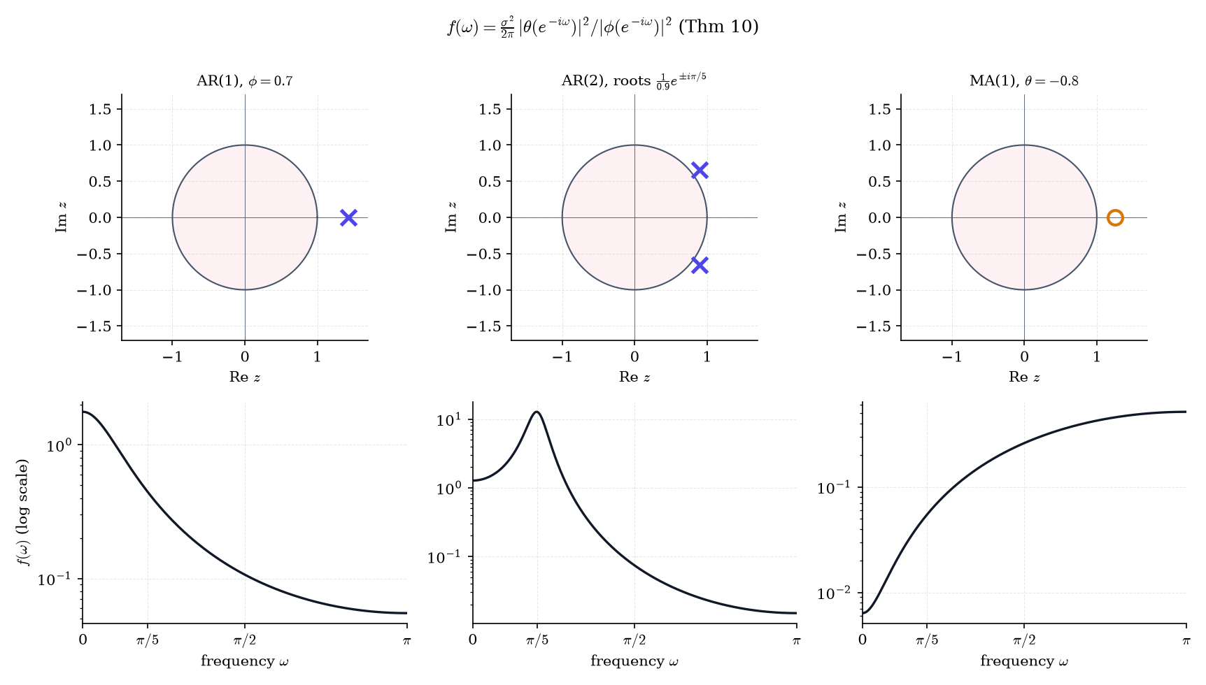
Example 15 Three spectra and their roots
AR(1), ϕ=0.7: a real root at 1/0.7, nearest e−iω at ω=0, so the spectrum is “red”: f(0)=1.76839 against f(π)=0.0550709.
AR(2) with roots 0.91e±iπ/5, that is, ϕ=(1.8cos(π/5),−0.81)=(1.456231,−0.81): a sharp peak at ω=0.6195, just below the root angle π/5=0.6283. The conjugate root’s pull shifts it slightly.
MA(1), θ=−0.8: a root at 1.25 puts the numerator near zero at ω=0, so the spectrum is “blue”: f(0)=0.0063662 against f(π)=0.515662.
Figure 7. The spectrum is a ratio of distances from the unit circle to the roots: AR roots near the circle make peaks, MA roots make troughs.
Example 16 The long-run variance is 2π f(0)
Set ω=0 in Definition 9: 2πf(0)=∑hγ(h)=σLR2, Theorem 2’s long-run variance. Theorem 11 then gives it in closed form, σLR2=σ2θ(1)2/ϕ(1)2. Topic 26’s chain (ϕ=0.9, σ2=0.19) gives 0.19/0.12=19, Example 4’s τ again. An ARMA(1, 1) with ϕ=0.7, θ=0.4 and σ2=1 gives 1.42/0.32=21.7778.
So the MCMC effective sample size is Nγ(0)/(2πf(0)): a chain is efficient when its spectrum has little mass at frequency zero.
Remark 18 Bochner, and Gaussian-process kernels as spectra
Herglotz’s theorem is the discrete-time case of Bochner’s theorem: a continuous stationary kernel k(τ) is positive definite if and only if it is the Fourier transform of a finite nonnegative measure (RAS2006 §4.2.1). Designing a GP kernel is designing a spectrum: the squared-exponential kernel has a Gaussian spectral density, the Matérn a Student-t-shaped one, and spectral-mixture kernels place Gaussian bumps where the periodogram peaks. See formalML: gaussian-processes and, for the operator view in which the Fourier basis diagonalizes a stationary covariance, formalML: spectral-theorem .
35.8 The periodogram and spectral smoothing
Replacing γ by γ^ in Definition 9 gives the periodogram, a cautionary tale.
The Fourier frequencies of a sample of size n are ωj=2πj/n. The periodogram (SCH1898) is
In(ωj)=2πn1t=1∑nxte−itωj2,
computed on the demeaned series (for j=0 demeaning changes nothing, as Proof 8 shows). Expanding the squared modulus as a double sum and grouping by lag gives In(ωj)=2π1∑∣h∣<nγ^(h)e−ihωj for j=0, the sample analogue of Definition 9, and Parseval’s identity reads n2π∑j=0n−1In(ωj)=γ^(0). We keep the 1/2π so that In and f live on one scale; Brockwell and Davis omit it. The Daniell estimator (DAN1946) averages 2m+1 neighboring ordinates,
f^m(ωj)=2m+11k=−m∑mIn(ωj+k),
with half-width m and bandwidthB=2π(2m+1)/n.
Theorem 12 The periodogram: asymptotically unbiased, never consistent
Let {Xt} be weakly stationary with mean μ, ∑h∣γ(h)∣<∞, and spectral density f. Let ωj=2πj/n∈(0,π).
(i) EIn(ωj)=2π1∑∣h∣<n(1−∣h∣/n)γ(h)e−ihωj, and if ωj(n)→ω∈(0,π) then EIn(ωj(n))→f(ω).
(ii) If the Xt are i.i.d. N(μ,σ2) (so f≡σ2/2π), then for every n the ordinates In(ωj), 0<ωj<π, are independent and each equals f⋅Ej with Ej∼Exp(1). In particular VarIn(ωj)=f2 for every n.
(iii) (Stated; BRO1991 Thm 10.3.2.) If Xt=μ+∑jψjεt−j with ε i.i.d., Eε4<∞, ∑j∣ψj∣∣j∣1/2<∞ and f>0, then for fixed 0<λ1<⋯<λk<π the vector (In(ωj1)/f(λ1),…,In(ωjk)/f(λk)), with ωji→λi, converges in distribution to i.i.d. Exp(1); and VarIn(ωj)→f(ω)2.
Proof 8 Proof of Thm 12 (i)–(ii) (The periodogram) [show][hide]
(i) For j≡0(modn), ∑t=1ne−itωj is a geometric sum of nth roots of unity and equals 0. So subtracting μ (or xˉ) from every observation leaves the Fourier sum unchanged, and
Take expectations and group by h=s−t exactly as in Proof 1:
EIn(ωj)=2π1∣h∣<n∑(1−n∣h∣)γ(h)e−ihωj.
Its distance from f(ωj)=2π1∑hγ(h)e−ihωj is at most 2π1[∑∣h∣<nn∣h∣∣γ(h)∣+∑∣h∣≥n∣γ(h)∣], which tends to 0 by Proof 1’s argument, uniformly in j. And f is continuous (a uniformly convergent series of continuous functions), so f(ωj(n))→f(ω).
(ii) Write Zt=(Xt−μ)/σ, i.i.d. N(0,1), and for 0<ωj<π set
Expanding the modulus, In(ωj)=2πnσ2[(∑tZtcostωj)2+(∑tZtsintωj)2]=4πσ2(Cj2+Sj2). The Cj,Sj are linear combinations of independent standard normals, hence jointly Gaussian with mean 0, and their covariances are the discrete orthogonality relations at Fourier frequencies: for 0<ωj,ωk<π,
each following from product-to-sum identities and the vanishing of ∑teitωm for m≡0(modn) (here m=j±k, and 0<j+k<n). So all the Cj,Sj are i.i.d. N(0,1), the ordinates are independent, and Cj2+Sj2∼χ22. Since χ22/2∼Exp(1),
In(ωj)=2πσ2⋅2Cj2+Sj2=f⋅Ej,Ej∼Exp(1),
so EIn(ωj)=f and VarIn(ωj)=f2, independent of n.
■ — using geometric sums of roots of unity, Proof 1’s Fejér-weight bound, discrete orthogonality of the trigonometric system, and the fact that uncorrelated jointly Gaussian variables are independent (Topic 8).
◼
More data buys more frequencies, not better estimates at each frequency. The periodogram uses n numbers to estimate about n/2 ordinates, so each one rests on two degrees of freedom forever — which is exactly why smoothing across neighbors restores consistency.
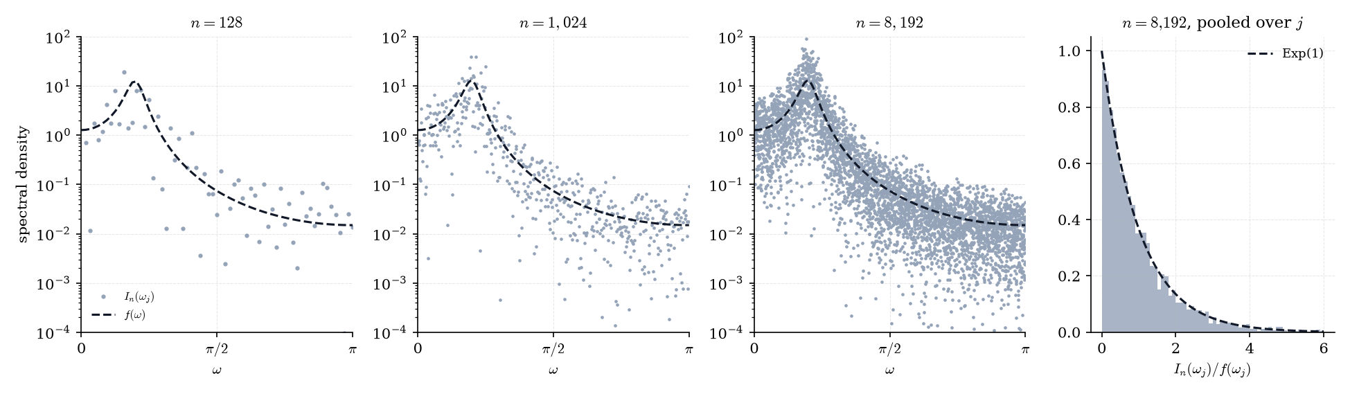
Figure 8. The raw periodogram never settles. Each ordinate is the spectral density times an Exp(1) variable, at every sample size.
For Example 15’s AR(2)-peak process, the pooled ratios In(ωj)/f(ωj) at n=8192 have mean 0.9988 and variance 1.0209, an Exp(1) as Theorem 12(iii) predicts. Repeated sampling at the fixed frequency j=n/8 (2,000 replications) gives VarI/f2=1.0753 at n=128 and 1.0365 at n=1024: no shrinkage.
Theorem 13 Consistency of the Daniell estimator (stated; BRO1991 Thm 10.4.1 and §10.4)
Under the conditions of Theorem 12(iii), if m=mn→∞ and m/n→0, then for 0<ω<π and ωj(n)→ω: Ef^m(ωj(n))→f(ω), Varf^m(ωj(n))∼f(ω)2/(2m+1)→0, hence f^m(ωj(n))Pf(ω). If f is twice continuously differentiable, the bias is approximately f′′(ω)B2/24, and the MSE-optimal half-width grows like m∝n4/5.
The variance is Theorem 12 again: 2m+1 nearly independent ordinates with variance near f2 average to f2/(2m+1). The bias is one Taylor expansion: averaging f over an interval of width B adds 2f′′⋅B1∫−B/2B/2u2du=f′′B2/24.
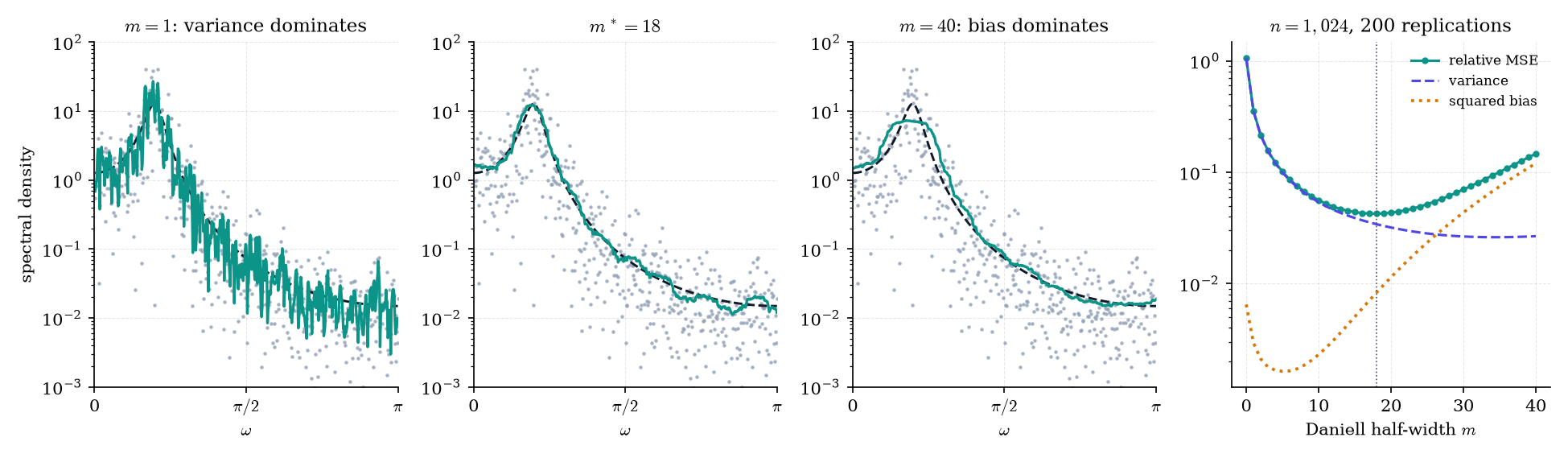
Figure 9. Smoothing the periodogram is a bandwidth problem: too little leaves noise, too much flattens the peak.
Over 200 replications at n=1024, the relative mean squared error N1∑j((f^−f)/f)2 is 1.063 for the raw periodogram (m=0), falls to its minimum 0.0425 at m∗=18 (bandwidth B∗=0.2270), and climbs back to 0.1469 at m=40 as the peak flattens. At a flat stretch of the spectrum (ω≈2.5), the relative variance tracks 1/(2m+1): 0.2081 against 0.2 at m=2, 0.0894 against 0.0909 at m=5, 0.0526 against 0.0476 at m=10.
Below, at m=0, push n from 128 to 8192: dots accumulate, the cloud doesn’t narrow. Then raise m until the estimate calms and the peak starts to sag; the bias–variance button reruns Figure 9’s right panel live.
Process:
Smoother:
bandwidth B = 2π(2m+1)/n = 0.0552relative SE ≈ 1/√(2m+1) = 0.333estimated peak ω = 0.6443, period 2π/ω = 9.75 steps
For a causal, invertible Gaussian ARMA with spectral density fβ, −2/n times the exact log-likelihood differs by oP(1) from n2∑j[logfβ(ωj)+In(ωj)/fβ(ωj)], summed over the Fourier frequencies in (0,π), plus a constant. Minimizing this Whittle objective gives an estimator with the same limit as the MLE (Theorem 8(b)).
Writing fβ=2πσ2gβ with g=∣θ∣2/∣ϕ∣2, the variance profiles out as σ^2=N2π∑jIn(ωj)/gβ(ωj) over the N frequencies, leaving Nlogσ^2+∑jloggβ(ωj) to minimize. One FFT makes each evaluation O(nlogn). Heuristically, the ordinates behave like independent f⋅Exp(1) variables, whose log-likelihood is exactly this sum.
Example 17 The sunspot spectrum
With n=309 the frequency grid has spacing 2π/309. The raw periodogram of the sunspot series peaks at a period of 11.04 years (j=28); the Daniell estimate with m=2 peaks at 10.3 years (j=30); the AR(2) spectrum of Example 12 peaks at 11.40 years. Three estimators, one solar cycle to within the grid’s resolution: at this n the grid, not the data, limits how finely the period can be located.
Remark 19 This is kernel density estimation in the frequency domain
Daniell is a uniform kernel smoother over frequencies, and Topic 30’s bandwidth analysis transfers: m plays the bandwidth h and 2m+1 plays nh. The variance ≈f2/(2m+1) matches KDE’s f(x)R(K)/(nh); the bias ≈f′′B2/24 matches h2f′′μ2(K)/2; balancing them gives an MSE-optimal m∝n4/5 and the familiar n−4/5 rate. Figure 9’s U-curve is Topic 30’s bandwidth figure in a new coordinate.
Remark 20 Lag windows, tapers, and multitaper
Smoothing in frequency is down-weighting γ^(h) in lag. The Bartlett window w(h)=1−∣h∣/M has variance ≈(2M/3n)f2, matching Daniell at M=3n/(2(2m+1)), the smoother’s toggle. Tapers reduce leakage from strong peaks; multitaper (THO1982) averages over orthogonal tapers instead of across frequencies.
Remark 21 HAC is spectral estimation at frequency zero
Newey–West (Remark 6) is a Bartlett lag-window estimate of 2πf(0), and choosing M is choosing a bandwidth. Example 1’s M=4 is far too narrow for ϕ=0.9, whose spectrum is sharply peaked at zero, so the estimate is biased low — hence coverage 0.621, not 0.95. Topic 26’s batch means (its Example 9) estimates the same 2πf(0).
35.9 GARCH: volatility from feedback
Topic 34’s Example 5 simulated two-regime market returns whose lag-1 autocorrelation was −0.018 but whose squared returns had lag-1 autocorrelation 0.206. To Wold it is white noise (Remark 7), yet its magnitude is predictable. Two mechanisms produce this fingerprint: a hidden regime that switches the variance (Topic 34’s HMM), or feedback, where a large move today raises tomorrow’s variance directly.
Definition 11 ARCH(q) and GARCH(1, 1)
Let zt be i.i.d. with mean 0 and variance 1, and set xt=σtzt, where the conditional varianceσt2 depends on the past. In an ARCH(q) model (ENG1982),
σt2=ω+i=1∑qαixt−i2,
and in a GARCH(1, 1) model (BOL1986),
σt2=ω+αxt−12+βσt−12,ω>0,α,β≥0.
(Here ω is the intercept, not a frequency; this section uses no frequencies.) The model is observation-driven: σt2 is a function of past observations, so the likelihood is an exact recursion.
Theorem 15 GARCH(1, 1) covariance stationarity
Let zt be i.i.d. with Ezt=0, Ezt2=1, and ω>0, α,β≥0. (i) If α+β<1, then
σt2=ω[1+k=1∑∞i=1∏k(αzt−i2+β)],xt=σtzt,
defines the unique strictly stationary GARCH(1, 1) solution with Ext2<∞ in which σt2 is a function of zt−1,zt−2,…; it is white noise with Var(xt)=ω/(1−α−β). (ii) Conversely, if a stationary solution with finite Ext2 exists, then α+β<1.
Proof 9 Proof of Thm 15 (GARCH(1, 1) stationarity) [show][hide]
Since xt−12=σt−12zt−12, the variance recursion is linear in σ2 with random coefficient At−1=αzt−12+β:
after iterating K times. The As are i.i.d., nonnegative, with EAs=α+β.
(i) Every term of the series St=ω[1+∑k≥1∏i=1kAt−i] is nonnegative and, by independence, E∏i=1kAt−i=(α+β)k. Monotone convergence gives ESt=ω/(1−α−β)<∞, so St is finite almost surely. Reindexing shows ω+At−1St−1=St, so σt2=St solves the recursion. St is one fixed measurable function of (zt−1,zt−2,…), so {(St,zt)} is strictly stationary, and St is independent of zt. Hence Ext=EStEzt=0, Ext2=EStEzt2=ω/(1−α−β), and for h>0, E[xtxt+h]=E[xtSt+h]Ezt+h=0, since zt+h is independent of everything dated earlier: white noise. For uniqueness, if σ~t2 is another such solution, then subtracting the iterated recursions,
using that ∏i≤KAt−i depends on zt−1,…,zt−K while the second factor depends only on earlier z‘s; so σ~t2=St almost surely.
(ii) If v=Ext2<∞ for a stationary solution, then Eσt2=v too (σt is independent of zt). Taking expectations in σt2=ω+At−1σt−12, with At−1 independent of σt−12,
v=ω+(α+β)v,sov(1−α−β)=ω>0,
which forces α+β<1.
■ — using the iterated recursion, independence of the zt, and monotone convergence (BOL1986; NEL1990).
◼
Example 18 Squared GARCH returns are an ARMA(1, 1)
Let νt=xt2−σt2, a martingale difference: E[νt∣past]=σt2E[zt2−1]=0. Substituting σt2=xt2−νt into the GARCH recursion gives
xt2=ω+(α+β)xt−12+νt−βνt−1,
an ARMA(1, 1) in xt2 with AR coefficient α+β and MA coefficient −β. When Ext4<∞ — for Gaussian zt, exactly when 3α2+2αβ+β2<1 — its ACF is
For the textbook values (ω,α,β)=(0.05,0.1,0.85): Var(xt)=1, ρx2(1)=0.17907, and ρx2(5)=0.145853. Topic 34’s HMM had squared-return autocorrelations decaying like λh; GARCH replaces that with (α+β)h−1.
Example 19 Fitting GARCH to hidden-regime data
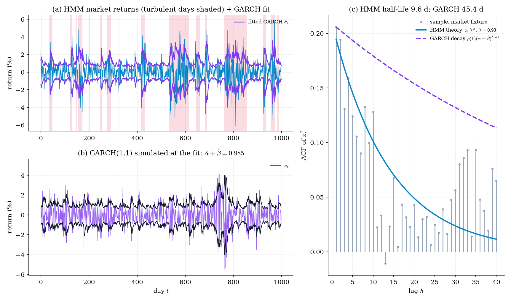
Fit Gaussian GARCH(1, 1) by quasi-maximum likelihood to Topic 34’s 1,000-day market fixture, which was simulated from the two-state HMM. The estimates are ω^=0.0803, α^=0.2821, β^=0.7028 (the arch package agrees to six decimals), so the persistence is α^+β^=0.9848 and the implied volatility half-life log0.5/log(α^+β^) is 45.4 days. The process that generated the data has a regime half-life of log0.5/log0.93=9.55 days.
Its unconditional variance ω^/(1−α^−β^)=5.30 is three times the sample variance 1.78, and 3α^2+2α^β^+β^2=1.129>1, so the fitted model has an infinite fourth moment and no squared-return ACF at all. The sample squared-return ACF at lags 1, 5 and 20 (0.206, 0.124, 0.043) tracks the HMM’s λh theory (0.1947, 0.1457, 0.0490). GARCH’s decay rate, scaled to the lag-1 value, would give 0.206, 0.194, 0.154 — far too slow. This is Lamoureux and Lastrapes’s lesson (LAM1990): regime shifts masquerade as near-integrated GARCH persistence.
Figure 10. GARCH fit to hidden-regime data. The fitted volatility persists far longer than the regimes that generated it.
Both models below give near-zero return autocorrelations and positive squared-return autocorrelations; they differ in the decay. Fit GARCH to an HMM path and watch α^+β^ land near 1.
Model:
Preset:
Remark 22 Observation-driven versus latent-state
GARCH’s variance is a function of past data, so its likelihood is an exact recursion; the HMM’s depends on a hidden state, so its likelihood needs the forward algorithm (Topic 34 §34.4). They differ in how volatility persists — geometric decay at rate α+β versus regime-length sojourns — and in reacting to one large shock: GARCH raises tomorrow’s variance at once, while the HMM waits for evidence of a switch.
Remark 23 Strict stationarity and IGARCH
Nelson (NEL1990) showed that GARCH(1, 1) has a unique strictly stationary solution if and only if Elog(αzt2+β)<0. By Jensen’s inequality this is weaker than α+β<1, and it allows the integrated case α+β=1 (IGARCH): strictly stationary, with infinite variance. Theorem 15’s condition is the stronger requirement that the variance be finite.
35.10 Connections and the road to Topic 36
Remark 24 MCMC diagnostics are spectral estimation
ESS is Nγ(0)/(2πf(0)) (Example 16); batch means, Geyer’s estimator, and spectral-variance estimators (Topic 26 §26.7) estimate 2πf(0) with three implicit bandwidths.
Remark 25 Dependent validation errors and time-series cross-validation
Backtest metrics and regret curves are dependent series: report HAC or block-bootstrap intervals (Remarks 6, 17), and use blocked or rolling-origin cross-validation so folds don’t interleave in time. Conformal guarantees need exchangeability that a series lacks; see formalML: conformal-prediction .
Remark 26 Linear state-space layers are learned ARMA filters
S4 (GU2022) and Mamba (GU2023) layers are discretized linear state-space models: their input–output map is a convolution with a rational transfer function — an ARMA-type filter — whose stability is a root condition (poles inside the unit circle in the z-transform convention, the reciprocal of §35.4’s). Mamba’s input-dependent coefficients break stationarity on purpose.
Remark 27 What we left out
VAR models, Granger causality and cointegration (HAM1994 Chs. 11, 19); long memory, where f(ω)→∞ at 0 (ARFIMA); nonlinear autoregressions; continuous-time CARMA; wavelets for nonstationary spectra (SHU2017 Ch. 4).
Remark 28 The road to Topic 36
Topic 36 writes an ARMA(p, q) in state-space form (Remark 10’s companion form) and runs the Kalman filter of Topic 34 §34.9 to get x^t and vt−1, evaluating Remark 8’s exact likelihood in O(n) and handling missing data for free; Kalman smoothing and EM follow. The notation here — ϕ, θ, σ2, γ, f, vn — carries over unchanged.