State-Space Models & Kalman Smoothing
Track 9's two halves turn out to be one object. Every ARMA model is a linear-Gaussian state-space model, and the Kalman filter's innovations are Wold's. Seven full proofs, featuring the Rauch–Tung–Striebel smoother. The exact likelihood is a product of innovation densities, computed in O(n), and missing data and forecasting cost nothing. Structural models become a modeling language, and EM's M-step is regression on smoothed moments. The steady-state Riccati equation explains why the gain settles. The Nile, Mauna Loa CO2 and Yule's sunspots are the data; O(n) Gaussian-process regression, recursive least squares, FFBS and S4 are the ML payoff. Track 9 closes here.
36.1 Motivation: one river, two views
One hundred years of annual Nile flow at Aswan, 1871–1970, in (COB1978), is the running example of Durbin and Koopman’s book (DUR2012), and it will be ours. The readings jump around, but something slower lies underneath: the level drops visibly around 1898, when work on the Aswan Low Dam began. Ask the question an ML practitioner would ask of any sensor log. What was the true level in 1913, given the noisy readings before and after it? The later readings carry information about 1913 because the level moves slowly. Using them is smoothing, the title half of this topic.
Topic 34 read a series like this as a hidden state seen through noise; Topic 35 read it through its autocovariance and its prediction errors. The Nile can be read both ways, and the readings agree. This topic explains why.
Model the unobserved level as a random walk and each reading as the level plus noise:
with all noise terms independent: a Gaussian random walk ( formalML: random-walks ) seen through measurement error. Here is the variance of the level’s yearly step and that of the measurement error (Durbin and Koopman’s and ). The maximum-likelihood estimates (§36.8) are and , so , with diffuse log-likelihood (Definition 5). Theorem 5 gives the distribution of each given all 100 readings; its mean falls from 1038.36 in 1897 to 951.00 in 1899 (Figure 1, left).
Difference the observations: , which is stationary, with autocovariances
An autocovariance that cuts off after lag 1 is the signature of an MA(1) (Topic 35 §35.5), with . So the hidden-level model is, from the observation-driven side, an ARIMA(0,1,1). At the MLE, ; the sample lag-1 autocorrelation of the 99 differences is , far outside the white-noise band . The MA coefficient is , where is the steady-state Kalman gain (§36.9, Example 15); as a check, .
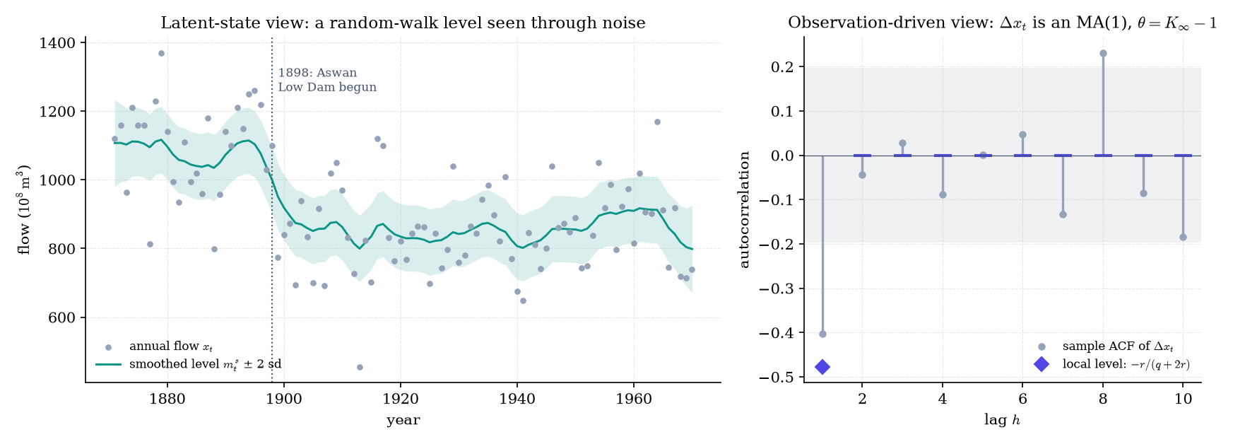
Figure 1. One series, two readings. As a hidden random-walk level seen through noise, the Nile drops after 1898; as an observation-driven model, its differences are an MA(1) with θ = K∞ − 1.
We write , and for expectation, variance and covariance, and for the Normal density with mean and covariance at (not Topic 34’s : is Topic 35’s AR coefficient). Bold letters stack over time. is a state-space sample length and an ARMA series length; they coincide in §36.4. Clashes are settled where they arise: the Kalman innovation versus Wold’s , the innovation variance versus Topic 35’s (equal, by Theorem 3), the covariance versus Topic 35’s projection (here ), and for the parameter vector, because is the MA coefficient.
Section 36.4 proves that the hidden-state and autocovariance descriptions coincide for every ARMA model, and §36.3 shows that the Kalman filter computes Topic 35’s prediction errors exactly and fast. Then every tool works on both: the smoother answers the 1913 question (§36.6), the exact likelihood costs (§36.3), missing data and forecasts are free (§36.5), and EM learns the parameters (§36.8).
36.2 The linear-Gaussian model, revisited
We work with the linear-Gaussian state-space model of Topic 34 §34.9 (Definition 8 there): a hidden state and an observation with
all mutually independent; is the observed value. Topic 34’s Theorem 12 (the Kalman filter) gives Gaussian predicted moments given and filtered moments given . From and :
Here is the innovation, its covariance and the gain; we cite the filter rather than re-prove it. Keep a geometric picture in mind: a Gaussian belief about a two-dimensional state is an ellipse, a level set of its density. Each step the dynamics carry it forward, the noise fattens it, and the observation cuts it down.
For data and the state :
- the predictive distribution is ;
- the filtering distribution is ;
- the smoothing distribution is , for ;
- the -step forecast distribution is , for .
Filtering is what we believe now; smoothing is what we believe in hindsight. Gaussianity of the last two is Theorems 4–5.
A constant-velocity tracker with state (position, velocity) observes position, with step :
Start from and .
- Predict. shears the ellipse (position picks up velocity), then inflates it: and .
- Update. We observe position . Then , , , and .
- Area (): 0.4472 → 0.6982 → 0.3204. Correlation: 0.408 → 0.732 → 0.442.
We observe only position, yet velocity’s variance shrinks too, from 0.7 to 0.404: the predict step correlated the coordinates, and the update slices the ellipse along the direction the observation sees, pulling the correlated direction along.
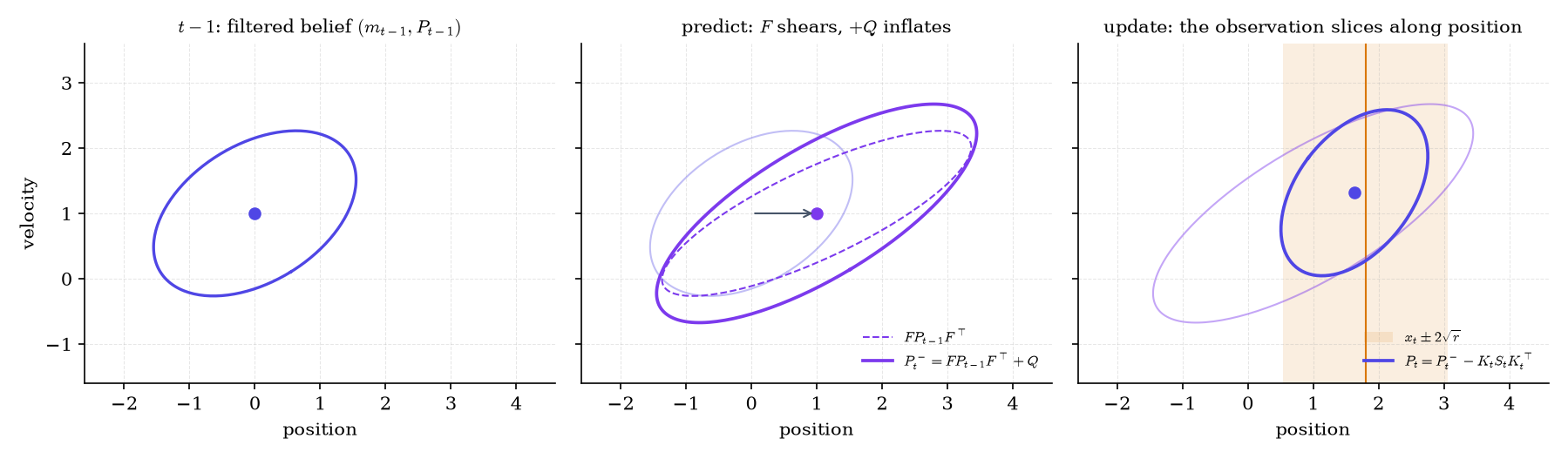
Figure 2. One Kalman step as geometry. The dynamics shear the belief and the noise inflates it; the observation slices it along the direction it sees, and the correlated direction shrinks too.
Step through the cycle, then switch Observe to velocity: the slice turns, and the position uncertainty grows without bound (§36.9).
Take a regression , , with examples arriving one at a time. Make the coefficients a state that never moves (, ), with time-varying observation row (Remark 5) and prior .
The filter mean after observations is the Bayesian linear regression posterior mean (Topic 25 §25.9), which is ridge regression with penalty ; as it becomes ordinary least squares (Topic 21 §21.4). With examples, three coefficients, and , the final filter mean differs from by at most , and matches to .
This is recursive least squares: online learning with exact uncertainty in per example for coefficients, and no refit. Setting lets the coefficients drift, the Kalman answer to concept drift.
Topic 34 delivered the filter and the predictive likelihood terms; the rest is new. The smoother of §36.6 is the continuous-state twin of §34.5’s forward–backward, and §36.8’s EM is the twin of §34.7’s Baum–Welch.
The proofs use . Code should use the Joseph form (JOS1968),
The two are algebraically identical (agreement on the Nile), but the Joseph form is a sum of positive-semidefinite terms, so rounding cannot destroy that property. Square-root filters propagate a Cholesky factor of ; information filters propagate , which suits vague priors; UD filters factor (SAR2013, AND1979).
Every result below holds verbatim with in place of , since only §36.9 uses time invariance. Examples 4 and 16 need this.
36.3 Innovations and the exact likelihood
Gram–Schmidt takes vectors in order and keeps from each only the part orthogonal to everything before it. Run it on in time order, with covariance as the inner product ( formalCalculus: hilbert-spaces ): the new part of is the innovation, Topic 35’s one-step prediction error (§35.3 Def 5), which Durbin–Levinson computes in . Orthogonal Gaussian pieces are independent, so the likelihood factors over innovations, which the filter computes in .
Let and be the Kalman innovations and innovation covariances, with every observed. Stack and let and . Then:
(i) The innovations are independent, with .
(ii) There is a unit lower block-triangular matrix (identity blocks on the diagonal) with . Hence with .
(iii) The log-likelihood is
and the filter evaluates it in operations.
Proof 1 Proof of Thm 1 (Prediction-error decomposition) [show]
Step 1: the innovations are a triangular affine function of the data. In Topic 34’s Theorem 12 the matrices , , , are computed from alone, never from the data. The means obey and , each an affine map of the previous mean and of . By induction on , is an affine function of :
for fixed vectors and matrices . Therefore
Stacking over , , where has identity blocks on its diagonal and zeros above it. Such a matrix is invertible with , and its inverse has the same form. Taking expectations, Step 2’s gives , so and .
Step 2: independence. Theorem 12 says that given , . Subtracting the conditional mean,
This conditional law does not depend on , so is independent of , and in particular . By Step 1, is an invertible function of , so conditioning on one is conditioning on the other. The chain rule then gives
which is (i): .
Step 3: factorization. From and the covariance rule for linear maps (Topic 8 §8.3), , which is (ii). Since ,
For the quadratic form, and , so
Substituting both identities into gives the formula in (iii).
Step 4: cost. One filter step forms in and in . It takes a Cholesky factor of in , the gain in , and the update in . That is per step and in total, against for a Cholesky factor of . — using Topic 34 Thm 12 (the filter and its predictive law), Topic 8 §8.3 (linear maps of Normal vectors), and the chain rule for densities.
Row of reads , with . This is Gram–Schmidt in the covariance inner product, run in time order, and is the block Cholesky factorization that Gram–Schmidt produces ( formalCalculus: linear-algebra ), one row at a time.
Theorem 1 holds for any . Starting the Nile filter from (Definition 5), the term () measures only the vague prior, so we drop it; at the diffuse log-likelihood is
- The innovation variance shrinks as the level is learned, from to .
- The innovations whiten the series. The lag-1 autocorrelation is 0.4984 for the flows and 0.1151 for the standardized innovations , and 4 of the 99 standardized innovations fall outside .
- For an ARMA(1,1), the factorization of Topic 35’s Toeplitz returns the Kalman on the diagonal of , to .
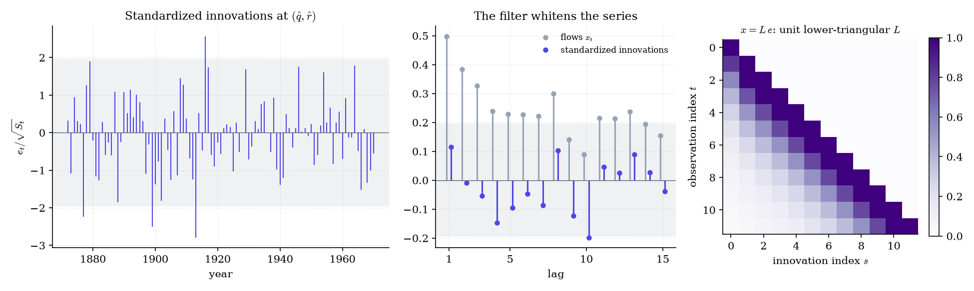
Figure 3. Innovations are Gram–Schmidt in time order. The filter turns an autocorrelated series into nearly white standardized errors, and the data are a unit-triangular mix of them.
Evaluating directly needs a Cholesky factor of a matrix: time, memory. The filter needs time and memory. For a 10,000-step sensor log that is infeasible versus instant; Example 16 shows the same gap for GP regression.
Under a correct model the standardized innovations are i.i.d. (Theorem 1(i)): they are the residuals. Check them with the sample ACF and its white-noise band (Topic 35 §35.6), a Ljung–Box statistic, and a Normal Q-Q plot. On the Nile, the run of large values after 1898 flags the level shift as an intervention (Remark 18). This is the residual check for any learned state-space or sequence model.
36.4 ARMA models are state-space models
Topic 35’s Remark 10 stacked an AR() into a first-order recursion with a companion matrix (§35.4). MA terms need one more idea: the state carries the part of each upcoming observation that the present already determines.
Let be an ARMA(, ) with i.i.d. . Let , and pad with for and for .
- is , with first column , ones on the superdiagonal, and zeros elsewhere.
- .
- and , with .
- So (rank 1) and : an observation with no noise.
- is the stationary covariance, the solution of .
For an ARMA(1,1), and
This is a noise-driven linear difference system ( formalCalculus: linear-systems ; HAR1989).
Let be an ARMA(, ) with i.i.d. , and take , , from Definition 2, with . Then:
(i) If and , the process satisfies .
(ii) A nonzero is an eigenvalue of if and only if . So the process is causal if and only if the spectral radius is below 1.
(iii) If the model is causal, (with ) has the unique solution . Started from , the observations have the law of consecutive values of the stationary ARMA, with autocovariance and .
Proof 2 Proof of Thm 2 (ARMA ⇔ state-space) [show]
(i) Write the state’s coordinates as , and set and . Row of the state equation reads
We claim that for each ,
For this is row itself. If it holds for at every time, substitute it (at time ) into row :
and the first two terms are the summand. At , using and the zero padding for and for ,
(ii) has first row and ones on the subdiagonal: it is Topic 35’s companion matrix (§35.4 Rem 10), zero-padded to size . and share eigenvalues. Take and . Rows of hold automatically: row of is . Row 1 reads . Dividing by gives , that is, .
Conversely, any eigenvector of with has this form. Rows force , so is a multiple of the vector above. So the nonzero eigenvalues are exactly the reciprocals of the roots of ; the padding contributes only zero eigenvalues. Causality (Topic 35 §35.4 Thm 5) is “every root of lies outside the unit circle”, which is .
(iii) If , pick . Then for some constant , so converges absolutely. Its sum satisfies
If and both solve the equation, satisfies for every , and the right side tends to 0. So the solution is unique.
The stationary causal ARMA is (Topic 35 Thm 5). Define , which converges in by the bound on . It satisfies , it is independent of , and
By (i), solves the ARMA equations. It is causal and stationary, so by the uniqueness in Topic 35 Thm 5 it equals , and matching coefficients of gives . Its state at any time is and independent of later shocks, which is exactly how Definition 2 starts . So the model started at produces the law of .
Finally, iterating the state equation times gives , and the sum is independent of . So , and
— using Topic 35 §35.4 Rem 10 (the companion matrix) and Thm 5 (causality; uniqueness of the causal solution), and convergence of geometrically dominated series.
Part (ii) keeps Topic 35’s Remark 10 promise: AR roots become eigenvalues, and causality becomes the stability condition ( formalCalculus: eigenvalues-eigenvectors , formalCalculus: stability-dynamics ). Part (iii) makes the filter, started at the stationary , compute the exact likelihood.
Here , , and the Lyapunov equation gives . Since , the first update pins the state to , and the filter then predicts with variance . So and for : the exact likelihood is the conditional likelihood plus one term for . For , .
Let be a causal, mean-zero ARMA(, ) driven by i.i.d. noise, filtered in the form of Definition 2 with the stationary of Theorem 2(iii). Write for the best linear predictor of from , and (Topic 35 Def 5, with and ). Topic 35 wrote this projection ; here is a covariance, so the projection is . Then for every :
(i) , so the Kalman innovation is the prediction error: .
(ii) .
(iii) If the model is also invertible, then , , and , where denotes the random innovation .
Proof 3 Proof of Thm 3 (Kalman innovations are Wold innovations) [show]
(i) By Theorem 2(iii), is a mean-zero Gaussian vector. Topic 34’s Theorem 12 gives , and by Step 1 of Proof 1 (with , so ) this is a linear combination of . The conditional expectation minimizes over all square-integrable functions of , so in particular over the linear span , and we have just seen that it lies in that span. By the projection theorem, the minimizer over a closed subspace is unique (formalCalculus: Hilbert spaces). Hence .
(ii) Theorem 12 also says that does not depend on . Taking expectations of the conditional mean-squared error, .
(iii) Invertibility gives with and (Topic 35 Thm 6). So
Causality makes uncorrelated with every , . Write
is a mean-square limit of linear combinations of past values, so , and Pythagoras gives
So and . For the upper bound, the truncated predictor lies in , and is the best element of that span, so
By Minkowski’s inequality in and ,
since the tail of a convergent series tends to 0. Combined with , we get . By (ii), and . — using Topic 34 Thm 12, Topic 8 §8.4 Thm 3 (Gaussian conditional means are linear), Topic 35 Def 5 and Thm 6, and the projection theorem.
The clash of Remark 1 is now a theorem: the innovation predicts from the finite past, the Wold innovation from the infinite past, and they agree in as . Topic 35’s Remark 8 follows: the exact Gaussian ARMA likelihood is a product of innovation densities, computed in .
Topic 35’s ARMA(1,1) fixture (, , ), demeaned, with every estimate evaluated under the exact likelihood:
| Estimator | exact at the estimate | |||
|---|---|---|---|---|
| Exact Gaussian MLE (Kalman, profile; 57 Nelder–Mead iterations) | 0.637421 | 0.404190 | 1.000176 | −1419.605827 |
| CSS (Topic 35) | 0.638968 | 0.402674 | 1.001488 | −1419.607146 |
| Whittle (Topic 35) | 0.641025 | 0.389910 | 1.011371 | −1419.678996 |
At all three are within one standard error of each other; Theorem 8’s asymptotic equivalence shows as contour-level agreement in Figure 4 (left). At the true parameters, the ratios for are 3.372549, 1.112558, 1.016187, 1.002549, 1.000407 and 1.000065, converging at the rate per step (Figure 4, right). See mode B of the explorer in §36.8.
Exact Gaussian MLE, mean estimated, on Yule’s sunspots (Topic 35 §35.6); the exact Kalman log-likelihood agrees with SARIMAX to :
| Model | |||||
|---|---|---|---|---|---|
| AR(2) | 49.659396 | (1.390656, −0.688571) | — | 274.760365 | −1307.318169 |
| ARMA(2,1) | 49.749208 | (1.470738, −0.755121) | −0.153691 | 270.878333 | −1305.138596 |
CSS gives AR(2) and ARMA(2,1) ; Whittle gives and .
- AR(2) innovation variances: and , then exactly 1 from on. CSS throws away precisely these two start-up terms (Remark 10).
- AIC vs BIC: with parameters, AIC prefers ARMA(2,1) (2620.28 vs 2622.64) and BIC prefers AR(2) (2637.57 vs 2638.94).
- Reconciliation: Topic 35’s table printed AR(2) from a slightly early-stopped optimizer; the exact optimum is .
This is the exact estimator that Topic 35’s Remark 14 deferred.
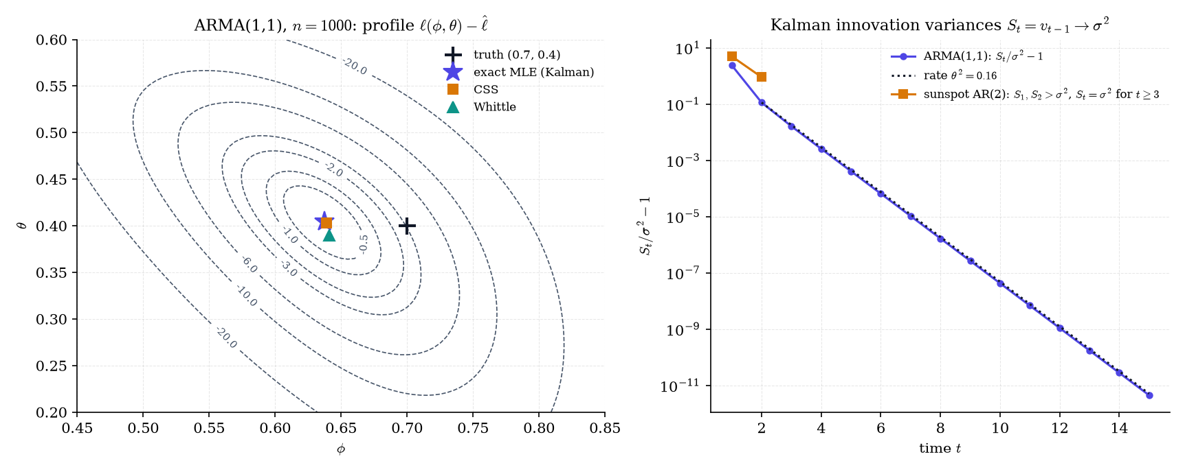
Figure 4. The exact ARMA likelihood, computed by the Kalman filter. CSS and Whittle land near its peak, and the innovation variances converge to σ² exactly as Theorem 3 predicts.
For invertible , gives the same observation process. Harvey’s, the companion and Akaike’s forms are similarity transforms of one another, so , , are unidentifiable without a canonical form (Remark 20).
Because and scale with , run the filter at to get and . Then and
This is the surface of Figure 4 and mode B, with one parameter fewer for Nelder–Mead.
CSS conditions on the first values and sets pre-sample shocks to zero. The exact likelihood keeps the start-up terms with : in total, but they matter when is small or roots are near the unit circle. They vanish geometrically, so all three estimators share a limit (Topic 35 Thm 8).
A unit root makes , and the Lyapunov equation has no solution. State-space methods handle ARIMA by differencing first or by a diffuse prior on the nonstationary states (Definition 5, §36.7, Remark 17).
36.5 Missing data and forecasting
In a state-space model a missing value is not a hole to patch but a step with nothing to update on.
Write for the set of times observed and for the observed values. At a time the filter skips the update, setting and , and adds no likelihood term. In code, a missing value is NaN.
Let be the observed times, and run the filter of Definition 3: at , set and and add no likelihood term. Then for every :
(i) and ;
(ii) , the log-density of the observed values alone;
(iii) the backward recursion of Theorem 5, run on these filtered moments, returns .
Proof 4 Proof of Thm 4 (Missing observations) [show]
Write . We prove (i) by induction on ; the base case is with .
Predict. Suppose . The noise is independent of and of every with , since those are functions of . So the predict step of Proof 10 in Topic 34 applies verbatim with the conditioning set in place of , giving the first half of (i). That argument never used which past observations were in the conditioning set.
Update. If , then : no new information arrives, the conditional law is unchanged, and setting , is exact. If , then is independent of . So given is jointly Gaussian with the covariance blocks of Proof 10, and the conditional MVN formula (Topic 8 §8.4 Thm 3) gives the usual update. That proves (i).
Likelihood. Order the observed times . The chain rule gives
and by the predict step and , each factor is , which is (ii). A missing time contributes no factor because it is not a variable of .
Smoother. Proof 5 uses three facts: the Markov property , restricted here to whichever of are observed; the filtered law from (i); and the linear-Gaussian dynamics. Each holds with in place of , so (iii) follows by the same argument. — using Topic 34 Proof 10 (predict and update), Topic 8 §8.4 Thm 3, the chain rule, and Theorem 5.
Delete Nile observations 21–40 and 61–80, leaving 60 values (DUR2012). With and no burn-in, the Kalman log-likelihood of the 60 observed values is −389.62213776, and the 60-dimensional brute-force Normal marginal gives the same number to . The diffuse gapped log-likelihood used for estimation is . This is the “missing data for free” of Topic 35’s Remark 28.
Append 20 missing years. The forecast mean stays flat at , and the state variance grows linearly, , with . The observation forecast standard deviation (sd) rises from 143.5235 () to 220.0145 (); the state sd at is 182.4776. The NaN-padded filter and the closed form agree to . Probabilistic forecasting with honest bands is a filter run past the data.
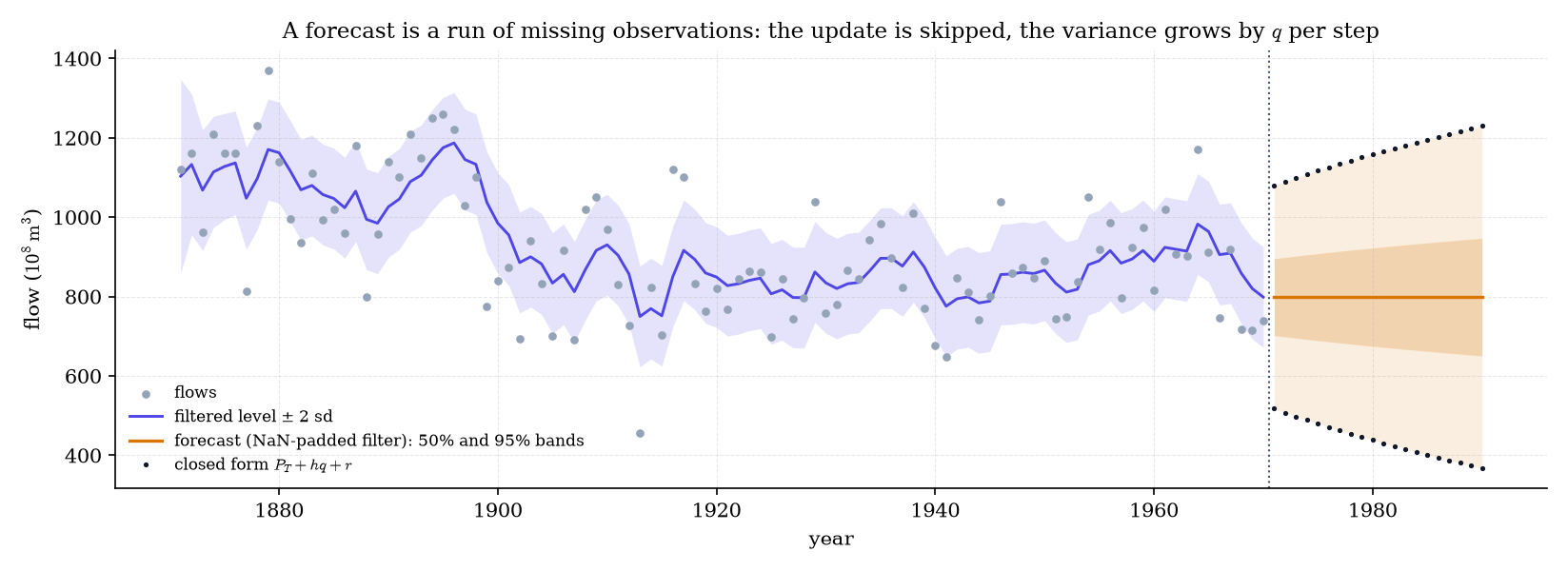
Figure 5. A forecast is a run of missing observations: the update is skipped and the variance grows by q each year.
If only some coordinates of are missing, drop those rows of and rows and columns of at that time (Remark 5). Irregular sampling is a time-varying and from a continuous-time model, as in Example 16.
Theorem 4 gives the likelihood of what was observed, which is the right one when missingness does not depend on the unobserved values (missing at random; JON1980). Sensor dropouts qualify; a reading censored because it was extreme does not.
36.6 Smoothing: the Rauch–Tung–Striebel recursion (featured)
Back to §36.1’s question. The filter at 1913 used only 1871–1913, but the later readings carry information too. Smoothing runs a second, backward pass that folds the future in: the continuous-state counterpart of §34.5’s forward–backward.
Run the filter on , and assume is invertible (true whenever ; Remark 15 covers the singular case). Set and , and for define the smoother gain and the recursion
Then for every , and the lag-one smoothed covariance is
Proof 5 Proof of Thm 5 (Rauch–Tung–Striebel smoother) [show]
Backward induction on . The case is the filter (Topic 34 Thm 12). Assume .
Step 1: the future enters only through . By Topic 34 Thm 4 (whose proof holds verbatim for densities), the joint density factors as
Group the factors that involve or , the single factor , and the factors that involve only and . Integrating out and conditioning on and leaves
because the last group does not involve and cancels in the normalization. The right side does not involve , so . Once we know , later observations tell us nothing more about .
Step 2: one backward conditioning. Given , and with independent. So the pair is jointly Gaussian with means and covariance blocks
The conditional MVN formula (Topic 8 §8.4 Thm 3), with block 1 = and block 2 = , gives
where the Schur complement was rewritten using .
Step 3: average over the smoothed . By Step 1, the law in Step 2 is also the law of given . Define
Given , , a law that does not depend on . So, given , is independent of , and
is an affine function of the Gaussian vector plus independent Gaussian noise. By Topic 8 §8.3 it is Gaussian, with mean and covariance
The same representation gives , since contributes nothing. Transposing yields . This completes the induction. — using Topic 34 Thm 4 (factorization, for densities), Topic 8 §8.4 Thm 3 (conditional MVN and the Schur complement), Topic 8 §8.3 (affine maps of Normals), and Topic 34 Thm 12 (the filter, for the base case).
The structure is §34.5’s forward–backward line for line. The filter supplies ; the backward pass multiplies in what the future says through one transition. The correction is how far hindsight moved our belief about tomorrow, and carries it back to today. In the scalar local level, , a weight between 0 and 1: small when the level was well pinned down at , and large when is small, so the level barely moves.
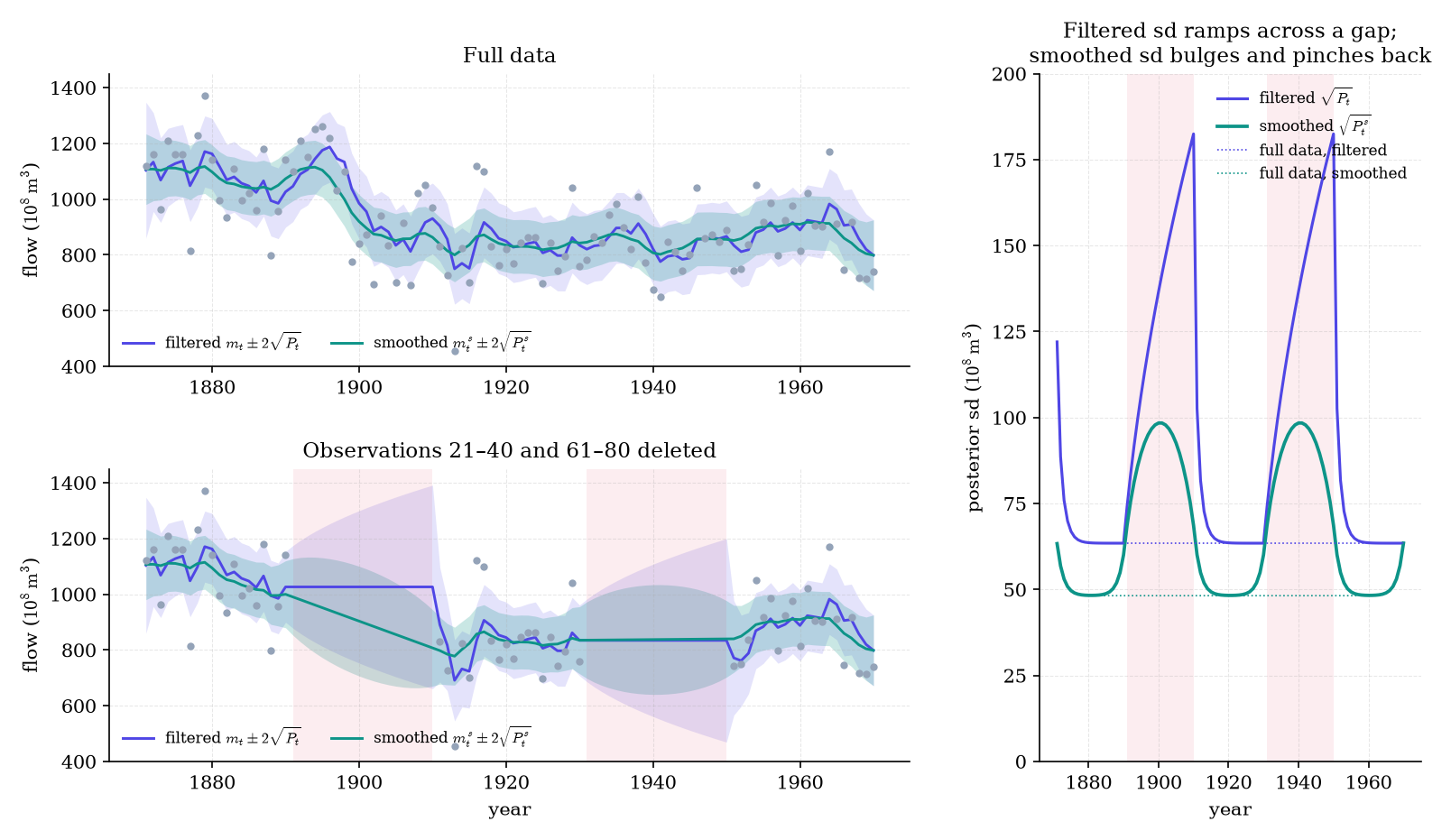
Figure 6. Filtering looks back; smoothing looks both ways. Across a gap the filtered band fans out and snaps shut, while the smoothed band bulges in the middle and pinches at the observations on either side.
Tap observations to delete them, or pick the gaps preset. Raise and both means chase the data; lower it and they flatten. The forecast slider is a gap at the end, and “MLE” refits .
With full data, the mid-sample filtered sd is 63.46 and the smoothed sd 48.20. The smoothed sd is 63.33 at and equals the filtered 63.46 at (no future to borrow). With Example 9’s gaps:
- the filtered sd ramps from 74.10 to 182.48 across the first gap;
- the smoothed sd bulges to 98.40 mid-gap and pinches to 68.65 at the gap’s first year and 60.08 at the last observed year before it.
The 1897-to-1899 level change is smoothed against filtered: the smoother spreads the 1898 shift symmetrically instead of reacting late.
The smoother gives marginals. For whole paths, say as one block of a Gibbs sampler, the same ingredients give exact joint draws.
Run the filter on . Draw , then for draw
Then is an exact draw from , at cost .
Steps 1 and 2 of Proof 5 are its two ingredients; the extension of Step 1 to is the same factorization argument.
With 2,000 FFBS draws at the MLE, the largest deviation of the draw mean from is 0.053 smoothed sds, and the average ratio of draw sd to is 1.0018. The explorer’s “Sample paths” toggle shows five draws, each a plausible history of the river’s level.
For Gaussian models the conditional mean is the projection (Topic 8 §8.4 Thm 3). So projects onto the span of , and onto the span of the whole sample, extending Topic 35’s projection picture (§35.3) from the past to the past and future. A larger subspace can only reduce error, so , with equality at ( formalCalculus: hilbert-spaces ).
Besides fixed-lag, fixed-point and two-filter smoothers, the disturbance smoother, which estimates and , is the efficient route to EM and outlier detection (DUR2012). If is singular, as in Harvey’s form, use the Moore–Penrose inverse; Proof 5 still holds.
Given the states, have conjugate inverse-gamma updates; given the variances, FFBS draws all states at once. Alternating is a blocked Gibbs sampler (Topic 26 §26.3) for West and Harrison’s dynamic linear models (WES1997; formalML: bayesian-inference ). Drawing the states jointly is what makes it mix.
36.7 Structural time-series models
Real series have trends that bend and cycles that repeat. State-space models write each feature as its own small component and add them: a modeling language in which we say what the series is made of, and the filter and smoother do the rest.
- Local level: state , with and .
- Local linear trend: state of level and slope, with and , so
- Dummy seasonal of period : the effect obeys , so that consecutive effects sum to noise. The state is , of dimension . has first row and the identity on its subdiagonal, and .
- Stacking: block-diagonal and , horizontally concatenated , and observation noise : a sum of independent, interpretable components (HAR1989, DUR2012).
Nonstationary components have no stationary start. We set with and drop the first log-likelihood terms, where is the number of diffuse states (1 for the local level, 13 for Example 13’s model). We call the result the diffuse log-likelihood. This is statsmodels’ default (loglikelihood_burn = k_states). The dropped terms are dominated by and carry essentially no information about the parameters.
Monthly means of the weekly Scripps flask record, March 1958 – December 2001 (; KEE2004, as bundled in statsmodels). The 5 months with no weekly sample are NaN, so Theorem 4 handles real missing data.
- Model: local linear trend plus a 12-month dummy seasonal, a 13-dimensional state.
- Fit: the maximum-likelihood variances (statsmodels’
UnobservedComponents) are irregular , level , slope and seasonal , with diffuse log-likelihood , which our own filter reproduces to . - Findings: the smoothed growth rate climbs from 1.006 ppm/yr in January 1960 to 1.545 ppm/yr in December 2000. The seasonal swing is 6.07 ppm from peak to trough. The smoother fills in the empty months.
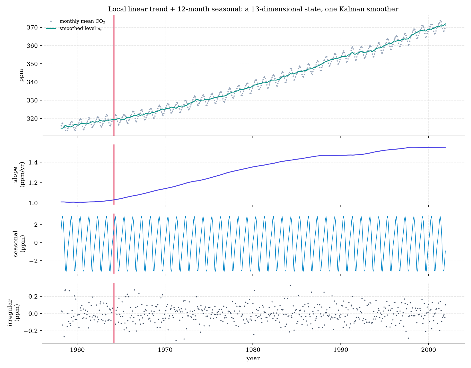
Figure 7. A structural model as a sum of interpretable parts: a slowly accelerating trend and a stable 6 ppm seasonal cycle in the Mauna Loa CO2 record.
Toggle components and move their variances; watch the badge when a toggle changes (Remark 21).
The honest limit is , where the naive filter loses precision; de Jong’s diffuse filter (DEJ1991) and Koopman’s exact initial filter (KOO1997) carry the and parts separately. For the scalar local level with prior mean 0 and variance , the first update gives
So the exact diffuse filter is “start at with variance , drop ”, which equals Definition 5 to . In general the diffuse part takes steps to clear.
The local linear trend’s reduced form is an ARIMA(0,2,2), and a seasonal block corresponds to seasonal differencing. A known break such as 1898 enters as a level-shift dummy, the canonical intervention analysis (DUR2012).
36.8 Learning the parameters: direct likelihood and EM
Direct maximization. Theorem 1 makes computable in , so any optimizer applies (Topic 14 §14.7). Nelder–Mead on , the same nelderMead Topic 35 ships, converges on the Nile in 60 iterations to , with diffuse . That is slightly higher than statsmodels’ default fit ( at , ), and Durbin and Koopman’s published give : a flat ridge (Figure 8).
EM. Treat the state path as missing data (Topic 14’s EM appendix, Topic 34 §34.7). For the linear-Gaussian model the M-step is closed-form.
Hold , , , fixed, let , and let all smoothed moments be computed under the current by Theorem 5. Write
for and . The EM objective is uniquely maximized over by
provided both right sides are positive definite. Combined with EM’s ascent property (Topic 34 §34.7 Thm 9), each iteration does not decrease .
Proof 6 Proof of Thm 7 (EM M-step) [show]
Step 1: the complete-data log-likelihood. By the factorization in Step 1 of Proof 5,
up to constants that do not involve . The first term does not involve either.
Step 2: conditional expectations. For a vector and a matrix , , and trace commutes with expectation. Expanding the outer product of and inserting and (Theorem 5) gives
Similarly, writing , the cross term has conditional mean zero, so
With and ,
The two brackets involve and separately, so we can minimize each one on its own.
Step 3: a matrix inequality. For a fixed , let over . Let be the eigenvalues of ; they equal those of the symmetric positive-definite matrix . Then
Each term is nonnegative, since for with equality only at . So , with equality exactly when every , that is, and .
Step 4: conclude. Applying Step 3 with and gives the unique maximizers and , the displayed formulas. — using Theorem 5 (smoothed means, covariances and lag-one covariances), the factorization of Topic 34 Thm 4, and Topic 34 §34.7 Thm 9 for ascent.
For the local level () the M-step reads
The squared residuals are the naive plug-in estimates; the and terms correct for the states being unobserved, Baum–Welch’s expected counts in continuous form. With missing data, averages over only (divide by ).
Start at , where . The first M-step moves to .
- After 172 iterations the relative-tolerance rule () stops EM at , , , still below the direct MLE.
- EM is within 0.01 of the maximum after 88 iterations, and every step increases ; the smallest increase is .
In Figure 8 the EM path climbs the contours and then crawls along the ridge: EM’s linear convergence, against Nelder–Mead’s 60 iterations. All log-likelihoods here are diffuse.
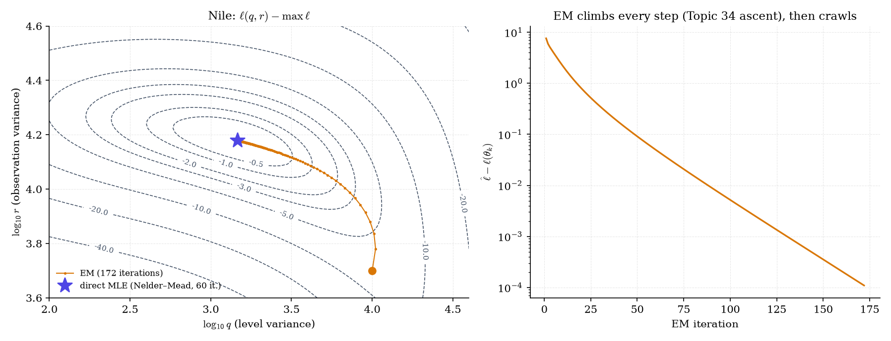
Figure 8. Two ways up the same hill. Direct maximization reaches the top in 60 iterations; EM climbs every step but crawls along the ridge.
Let parameterize a stationary SSM, with and the observation law depending smoothly on . Assume the model is identifiable, the truth is interior, and the per-observation information
is nonsingular. Then the MLE is consistent and .
This is Topic 14 §14.5’s theorem for dependent data, with the score built from innovations; Topic 35’s Theorem 8 is the ARMA case. Variances on the boundary (: a level that never moves) have nonstandard limits.
The variances are hyperparameters of a Gaussian prior on the state path, and is a marginal likelihood. Maximizing it is Topic 28 §28.7’s Type-II MLE and Topic 33’s empirical Bayes: the data choose the smoothing strength , as evidence maximization chooses GP kernel hyperparameters.
- EM’s rate is set by the fraction of missing information (here, of the state path), which is why Example 14 crawls. Practitioners run EM to get close, then switch to quasi-Newton.
- With and free, the M-step is two regressions on smoothed moments: and . Remark 8’s similarity transforms make that model unidentifiable without constraints.
- Subspace methods such as N4SID estimate without likelihood iterations; HAN1988 gives the theory.
Use AIC or BIC (Topic 24 §24.3, §24.4) with free variances. Diffuse log-likelihoods with different numbers of diffuse states drop different numbers of terms, so compare them only via the exact diffuse likelihood (Remark 17) or on a common burn-in; comparing them directly is a common silent error.
Mode A is Figure 8’s surface: tap to start EM anywhere and watch every increase stay positive. Mode B is §36.4’s exact ARMA(1,1) surface with the exact, CSS and Whittle optima; at they spread apart.
36.9 The steady state: Riccati, observability, and the constant gain
In Topic 34’s Example 15 the local-level gain settled to from step 22 on. Since and never depend on the data, why and how fast it settles is a property of a deterministic map, the Riccati recursion.
Let and , and define on . The local level’s predicted variances obey (Topic 34 Ex 15). Then for any :
(i) has exactly one fixed point in , namely .
(ii) With ,
so geometrically.
(iii) whenever , and the gains satisfy , so they converge at the same rate.
Proof 7 Proof of Thm 9 (Convergence of the scalar Riccati recursion) [show]
(i) For , means , that is,
The two roots multiply to , so exactly one is positive: .
(ii) For ,
Take and , and use (the ‘s cancel):
Since , the first factor is at most 1, and the second equals . This gives the inequality. Iterating, , because .
(iii) By (ii), , so the ratio . For the gains, with ,
whose absolute value is at most , because . — using Topic 34 Ex 15 (the Riccati recursion and its fixed-point equation) and elementary algebra.
For and the asymptotic rate is per step, so loses a factor of 10 roughly every 3.6 steps. That is why Topic 34 saw the gain settle within by step 22. The uniform rate in (ii) holds from the first step, whatever the prior variance.
For and : and : Topic 34’s values, now to nine digits.
- Rate: Theorem 9(iii) predicts the asymptotic contraction ; the measured log-linear rate of is 0.532363.
- Nile at the MLE: , rate 0.537947 (Example 2’s ).
- Matrix case: for Example 3’s tracking model the gain converges to , with
That solves the discrete algebraic Riccati equation (agreement after 22 iterations), reached from and alike.
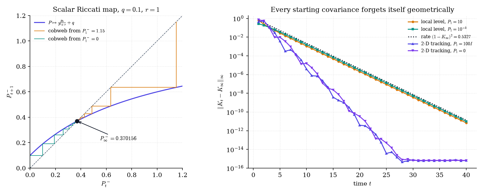
Figure 9. Why the gain settles. The Riccati map contracts toward its fixed point, and every starting covariance is forgotten at a geometric rate.
In more dimensions the question is whether, not just how fast: a state direction the data never see has nothing to pin it down.
- is observable if the matrix stacking has rank : every direction of the state eventually shows up in the data.
- is controllable, where , if the matrix placing side by side has rank : noise eventually reaches every direction.
- Detectable and stabilizable weaken these to “every unstable mode” (eigenvalues ).
Constant velocity with position observed is observable: the rank-2 matrix stacks and . With velocity observed, , and the unstable position mode is not detectable.
Let and , and suppose is detectable and stabilizable (Definition 6). Then the discrete algebraic Riccati equation
has a unique positive-semidefinite solution . For every the predicted covariances converge to it, and the steady-state closed-loop matrix has spectral radius less than 1.
Theorem 9 is the case with an explicit rate, and is its closed-loop factor. In §36.2’s stepper, “Run to steady state” converges in about 20 steps with position observed and never with velocity alone, where detectability fails.
Once , the filter is the time-invariant recursion : the Wiener filter, exponential smoothing for the local level (Topic 34 Ex 15), and the invertible AR() predictor of Theorem 3(iii) for an ARMA. Production systems often precompute ; the price is a slightly wrong start-up transient, exactly Remark 10’s CSS-versus-exact difference.
For observed continuously through with white noise, the Riccati recursion becomes the Riccati ODE
(KAL1961; formalCalculus: first-order-odes ). Its steady state solves the continuous algebraic Riccati equation, .
36.10 Connections, and the Track 9 synthesis
Exact GP regression on points costs . On a line, for the Matérn family, the state-space view removes that cost.
The kernel , with divided by the length scale, is the covariance of the stationary solution of for the state , where
and is a Brownian motion (HAR2010).
- Exact discretization: between inputs a gap apart,
with ; irregular inputs give a different and at each step (Remark 5), and .
- Setup: 60 irregular inputs on , , length scale 1.5 (so ), and noise variance . The RTS smoother’s posterior mean equals the Cholesky GP posterior mean to , and its variance to .
- Cost: fitted log-log slopes of runtime against are 2.6 (dense) and 1.0 (Kalman); absolute timings are machine-dependent, and the gap widens with .
Exact one-dimensional GP regression is an smoothing problem, and every half-integer Matérn- kernel works the same way with states ( formalML: gaussian-processes ).
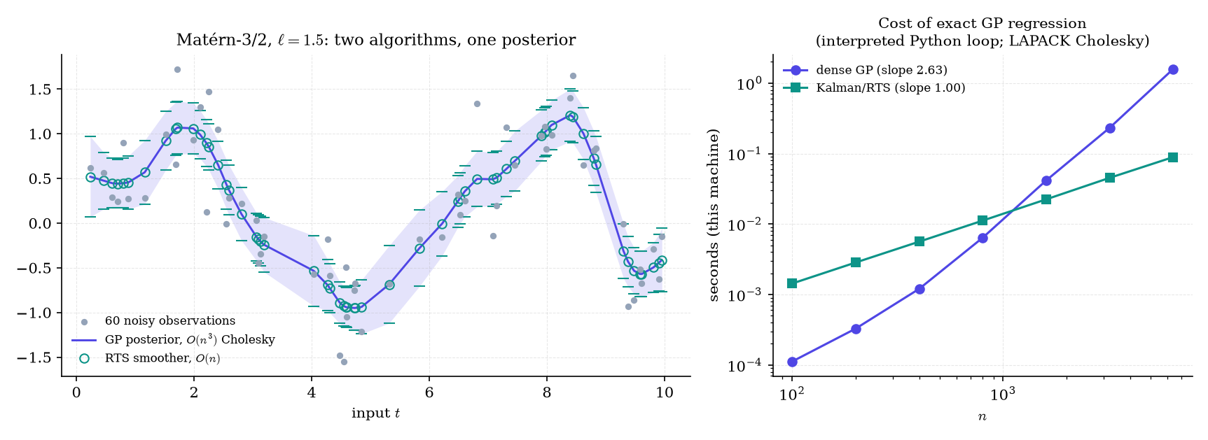
Figure 10. A Matérn Gaussian process is a two-state linear model, so the Kalman smoother returns the exact GP posterior in linear time.
This extends Topic 34’s Remark 25. S4 (GU2022) discretizes a continuous linear system exactly as Example 16 does, , and runs the state equation as a learned, noise-free layer. Mamba (GU2023) makes , and the output map input-dependent. What they omit is everything this topic adds: a noise model, a likelihood, uncertainty bands, smoothing, and principled handling of missing tokens.
This extends Topic 34’s Remark 22. With nonlinear or , the extended and unscented filters linearize; the smoother then needs the same linearization backward (the extended RTS smoother), and EM needs Monte Carlo or variational E-steps ( formalML: variational-inference ). Particle filters (GOR1993) and particle smoothers replace every Gaussian closed form with weighted samples, and FFBS (Theorem 6) is the exact linear-Gaussian case of backward-simulation smoothing ( formalML: sequential-monte-carlo ).
Three topics, one object. Topic 34 built a hidden chain and got filtering, smoothing and EM on a trellis. Topic 35 built a stationary series from its autocovariance and got Wold’s innovations and the spectrum. This topic proved they meet: an ARMA is a linear-Gaussian SSM, its innovations are Kalman’s, and the exact likelihood, smoother and EM are the continuous-state versions of Topic 34’s recursions. The road forward runs to formalML ( formalML: gaussian-processes , formalML: sequential-monte-carlo , formalML: bayesian-inference ). This closes Track 9, not the site: Track 8’s Parametric vs Nonparametric Models is still to come.
References
- Durbin, James, and Siem Jan Koopman. (2012). Time Series Analysis by State Space Methods (2nd ed.). Oxford University Press.
- Harvey, Andrew C. (1989). Forecasting, Structural Time Series Models and the Kalman Filter. Cambridge University Press.
- Särkkä, Simo. (2013). Bayesian Filtering and Smoothing. Cambridge University Press.
- Brockwell, Peter J., and Richard A. Davis. (1991). Time Series: Theory and Methods (2nd ed.). Springer.
- Shumway, Robert H., and David S. Stoffer. (2017). Time Series Analysis and Its Applications: With R Examples (4th ed.). Springer.
- Kalman, Rudolph E. (1960). A New Approach to Linear Filtering and Prediction Problems. Journal of Basic Engineering, 82(1), 35–45.
- Rauch, Herbert E., F. Tung, and Charlotte T. Striebel. (1965). Maximum Likelihood Estimates of Linear Dynamic Systems. AIAA Journal, 3(8), 1445–1450.
- Shumway, Robert H., and David S. Stoffer. (1982). An Approach to Time Series Smoothing and Forecasting Using the EM Algorithm. Journal of Time Series Analysis, 3(4), 253–264.
- Dempster, A. P., N. M. Laird, and D. B. Rubin. (1977). Maximum Likelihood from Incomplete Data via the EM Algorithm. Journal of the Royal Statistical Society, Series B, 39(1), 1–22.
- Jones, Richard H. (1980). Maximum Likelihood Fitting of ARMA Models to Time Series with Missing Observations. Technometrics, 22(3), 389–395.
- Carter, C. K., and R. Kohn. (1994). On Gibbs Sampling for State Space Models. Biometrika, 81(3), 541–553.
- Frühwirth-Schnatter, Sylvia. (1994). Data Augmentation and Dynamic Linear Models. Journal of Time Series Analysis, 15(2), 183–202.
- de Jong, Piet. (1991). The Diffuse Kalman Filter. Annals of Statistics, 19(2), 1073–1083.
- Koopman, Siem Jan. (1997). Exact Initial Kalman Filtering and Smoothing for Nonstationary Time Series Models. Journal of the American Statistical Association, 92(440), 1630–1638.
- Anderson, Brian D. O., and John B. Moore. (1979). Optimal Filtering. Prentice-Hall.
- Hannan, E. J., and Manfred Deistler. (1988). The Statistical Theory of Linear Systems. Wiley.
- Bucy, Richard S., and Peter D. Joseph. (1968). Filtering for Stochastic Processes with Applications to Guidance. Interscience.
- Kalman, Rudolph E., and Richard S. Bucy. (1961). New Results in Linear Filtering and Prediction Theory. Journal of Basic Engineering, 83(1), 95–108.
- Hartikainen, Jouni, and Simo Särkkä. (2010). Kalman Filtering and Smoothing Solutions to Temporal Gaussian Process Regression Models. 2010 IEEE International Workshop on Machine Learning for Signal Processing, 379–384.
- West, Mike, and Jeff Harrison. (1997). Bayesian Forecasting and Dynamic Models (2nd ed.). Springer.
- Gordon, N. J., D. J. Salmond, and A. F. M. Smith. (1993). Novel Approach to Nonlinear/Non-Gaussian Bayesian State Estimation. IEE Proceedings F, 140(2), 107–113.
- Gu, Albert, Karan Goel, and Christopher Ré. (2022). Efficiently Modeling Long Sequences with Structured State Spaces. International Conference on Learning Representations (ICLR 2022).
- Gu, Albert, and Tri Dao. (2023). Mamba: Linear-Time Sequence Modeling with Selective State Spaces. arXiv preprint arXiv:2312.00752.
- Cobb, George W. (1978). The Problem of the Nile: Conditional Solution to a Changepoint Problem. Biometrika, 65(2), 243–251.
- Keeling, Charles D., and Timothy P. Whorf. (2004). Atmospheric CO2 Concentrations Derived from Flask Air Samples at Sites in the SIO Network [Data set]. In Trends: A Compendium of Data on Global Change. Carbon Dioxide Information Analysis Center, Oak Ridge National Laboratory.