Random Variables & Distribution Functions
The bridge from events to numbers — PMFs, PDFs, CDFs, and the distribution machinery that makes statistical computation possible
1. Random Variables: The Bridge from Events to Numbers
In Topic 1 and Topic 2, we worked entirely with events — subsets of the sample space . We asked questions like "" and "". But most of statistics and machine learning works with numbers, not sets. We want to talk about the “value” of a die roll, the “height” of a person, the “loss” of a model.
A random variable is the bridge. It’s a function that assigns a number to each outcome.
Motivating example. Roll two dice. The sample space is with 36 outcomes. Define by . Now instead of asking “what is the probability of outcomes in the set ?” we simply ask "". The random variable compresses the 36-element sample space into the numbers .
This is not just notational convenience — it’s a change of mathematical universe. Once we have a function , we can add random variables (), multiply them, take expectations (), compute variances (), and apply calculus. The entire toolkit of analysis opens up.
Let be a probability space. A random variable is a function that is measurable with respect to — meaning that for every Borel set ,
In practice, the condition we check most often is the CDF condition: for every ,
This is sufficient because the half-lines generate the Borel -algebra (see Topic 1, Example 4).
The measurability condition ensures that we can assign a probability to every statement of the form "" or "". Without it, is undefined — the set might not be in , and only speaks to events in . For finite or countable sample spaces with the discrete -algebra (the power set), every function is measurable — so the condition is automatic. It only becomes restrictive for uncountable , and even then, every function you’ll encounter in practice is measurable.
Why this matters for ML: When you write ”,” you are implicitly working with the Borel -algebra on . The measurability requirement — that a random variable must pull Borel sets back to events in your -algebra — is what makes statements like "" well-defined. We formalized -algebras in Topic 1.
A random vector is a function where each component is a random variable.
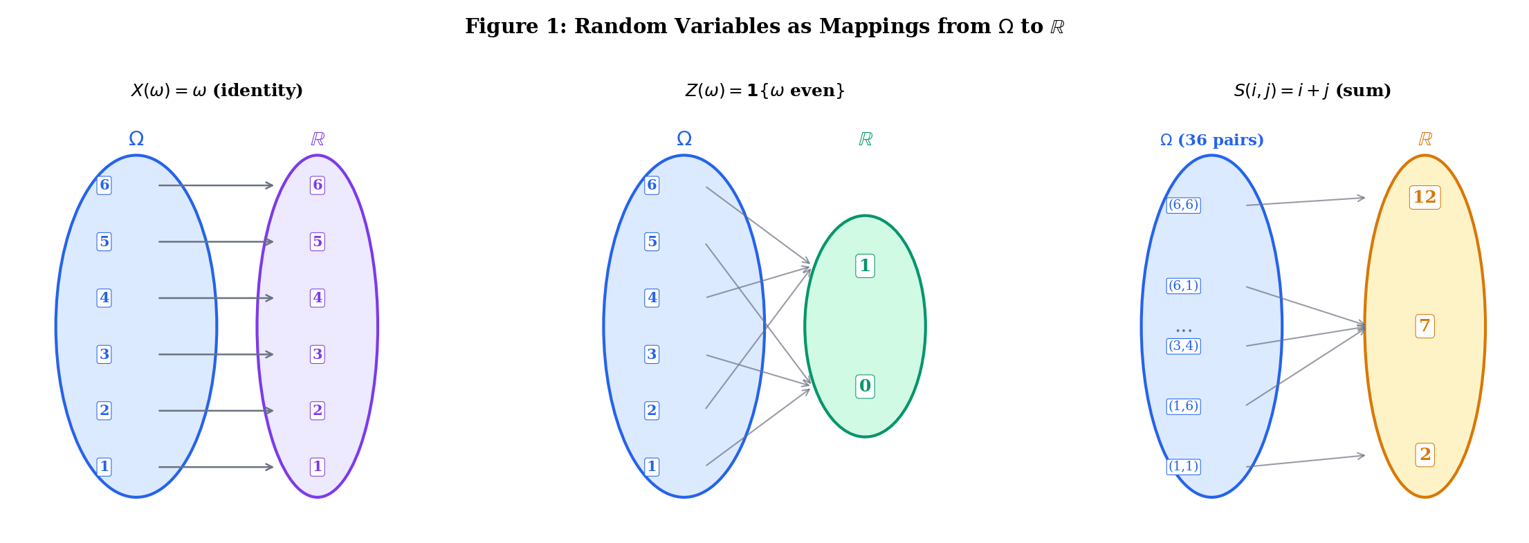
Roll one die. , . The identity function is a random variable. So is , or (the indicator of “even”). Each creates a different mapping from outcomes to numbers.
, . The pre-images are:
- , so
- , so
- , so
The random variable induces a probability distribution on via the pre-image and .
Use the explorer below to see how random variables map outcomes to numbers. Select an experiment and a mapping, then watch the arrows and the induced probability distribution:
| Value x | Pre-image X⁻¹({{x}}) | P(X = x) |
|---|---|---|
| 1 | {1} | 1/6 = 0.1667 |
| 2 | {2} | 1/6 = 0.1667 |
| 3 | {3} | 1/6 = 0.1667 |
| 4 | {4} | 1/6 = 0.1667 |
| 5 | {5} | 1/6 = 0.1667 |
| 6 | {6} | 1/6 = 0.1667 |
2. Discrete Random Variables and PMFs
A random variable is discrete if it takes values in a finite or countably infinite set .
The distribution of a discrete random variable is completely described by its probability mass function.
The probability mass function (PMF) of a discrete random variable is the function defined by
The PMF satisfies two properties:
- for all (from Axiom 1 of the Kolmogorov axioms, Topic 1)
- (from Axiom 2, summing over all values in the support)
The support of a discrete random variable is the set of values where the PMF is positive:
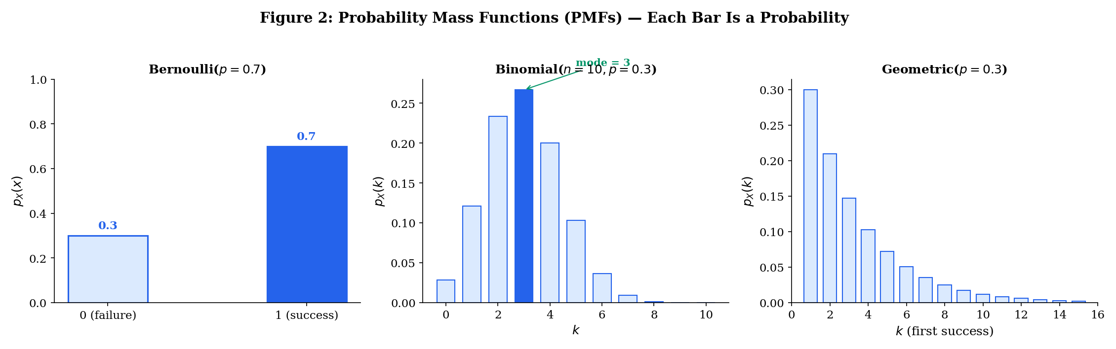
A Bernoulli random variable models a single trial with two outcomes. with and for some . Written compactly:
We write . This is the building block of classification: "" is logistic regression.
The sum of independent trials. with
We write . The binomial coefficient counts the number of ways to arrange successes among trials — this is the combinatorics from Topic 1 (§6) in action.
For a discrete random variable, is an actual probability. This is NOT true for continuous random variables (as we’ll see in §3). The probability of any event involving is computed by summing the PMF:
3. Continuous Random Variables and PDFs
When the sample space is uncountable — say — a random variable can take any real value in a continuum. For any specific value , we have . This is not a pathology; it’s a fundamental feature of the uncountable. There are uncountably many possible values, and since they must sum to 1, each individual probability must be zero.
So we can’t describe continuous random variables with a PMF. Instead, we describe them with a density — a function whose integral gives probabilities.
A random variable is continuous if there exists a non-negative function such that for every interval ,
The function is called the probability density function (PDF). It satisfies:
- for all
These mirror the PMF conditions — replace sums with integrals.
This is perhaps the most common confusion in probability. For a continuous random variable:
- is a density, not a probability. It can be greater than 1.
- is (informally) the probability that falls in a tiny interval around .
- Only integrals of the density give probabilities.
- for every individual . Probabilities of intervals are what matter.
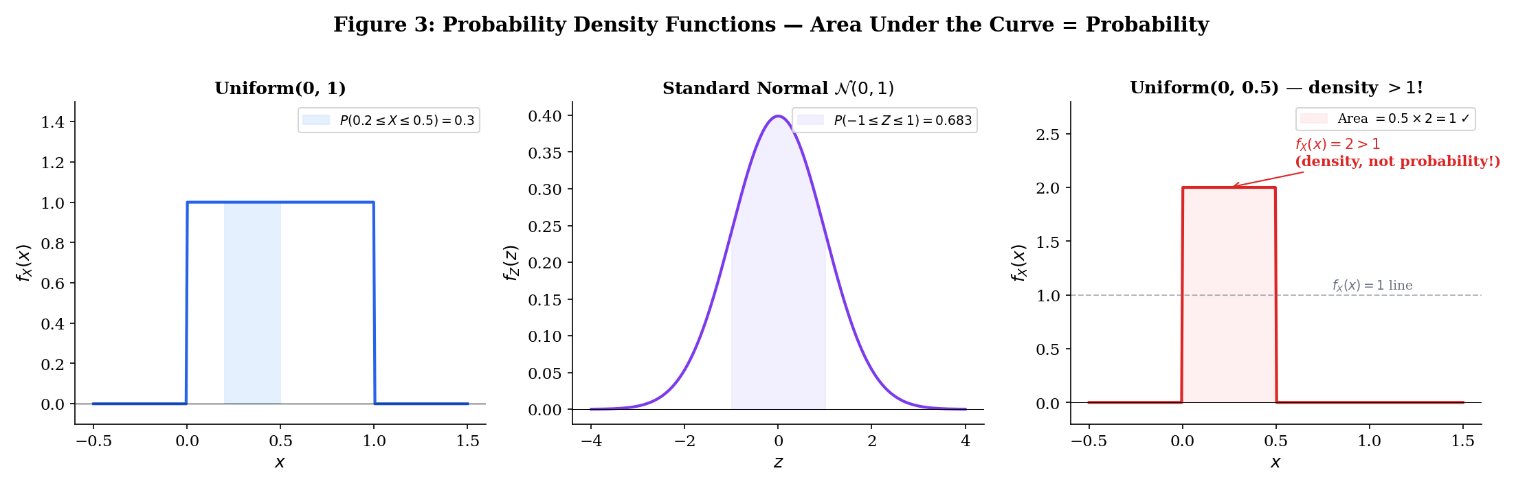
has density for and otherwise. Then . The probability equals the length of the interval — probability is area under the density curve.
has density
This density is positive everywhere on and integrates to 1 (a non-trivial fact requiring the Gaussian integral ).
Note that — this is less than 1 in this case, but for a distribution, on , which exceeds 1. The density is not bounded by 1.
Toggle between discrete and continuous modes in the explorer below. In discrete mode, each bar height IS a probability. In continuous mode, drag to select an interval — the shaded AREA is the probability:
Click a bar to see its probability value
4. The Cumulative Distribution Function
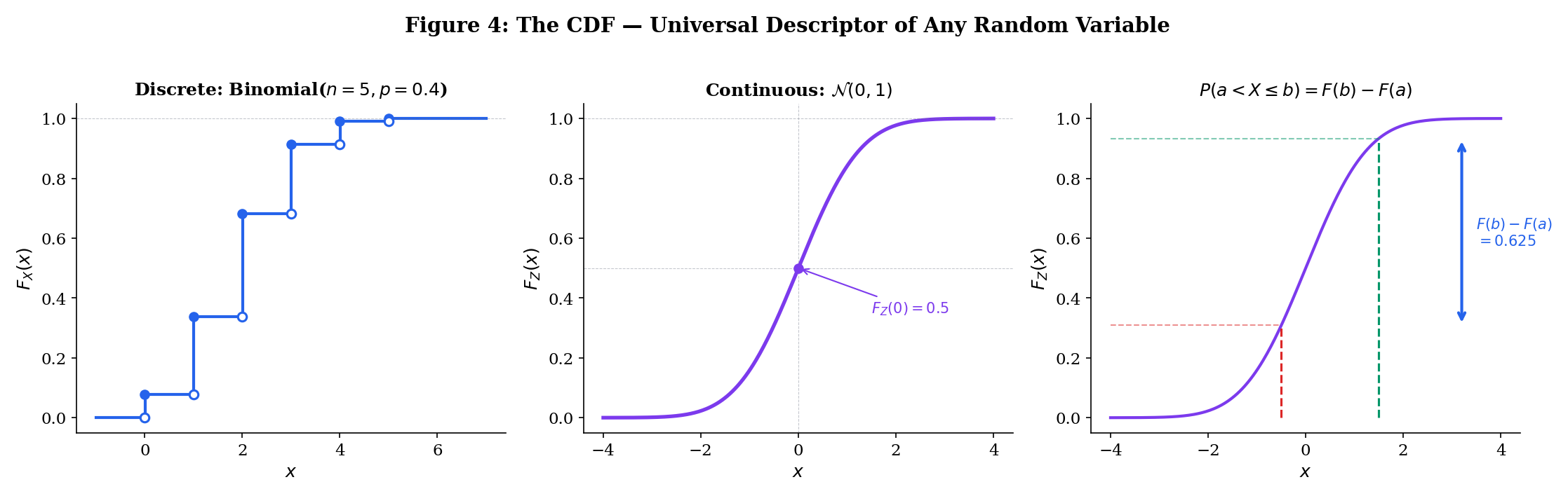
The CDF works for every random variable — discrete, continuous, or mixed. It is the universal descriptor.
The cumulative distribution function (CDF) of a random variable is
For any random variable , the CDF satisfies:
- Non-decreasing: If , then .
- Right-continuous: for all .
- Limits at infinity: and .
Proof Properties of the CDF (Theorem 1) [show]
(1) If , then . By monotonicity of probability (Topic 1, Theorem 2): .
(2) Let . Then the events decrease to . By continuity of probability from above (Topic 1, Theorem 6b):
i.e., .
(3) For , , so by continuity from above. For , , so by continuity from below.
The limit properties rely on the convergence framework from formalCalculus: Sequences & Limits .
The CDF gives us a direct route to probabilities of intervals:
This follows from (disjoint).
For continuous random variables, , so strict/non-strict inequalities don’t matter: .
For discrete random variables, the CDF is a step function — it jumps at each value in the support. The jump at has height .
For a continuous random variable with PDF :
And by the fundamental theorem of calculus, wherever is continuous:
The PDF is the derivative of the CDF. The CDF is the antiderivative of the PDF. This connection requires the integration and differentiation machinery from formalCalculus: Change of Variables .
Explore discrete (step function) and continuous (smooth curve) CDFs side by side. Drag the vertical line to query :
5. Joint Distributions
In ML, we almost never work with a single random variable. A feature vector is a collection of random variables. Understanding the joint behavior — how they relate to each other — is essential.
For discrete random variables and , the joint PMF is
It satisfies and .
For continuous random variables and , the joint PDF is a function such that
for every (measurable) set . It satisfies and .
The joint CDF is
This works for any pair of random variables.
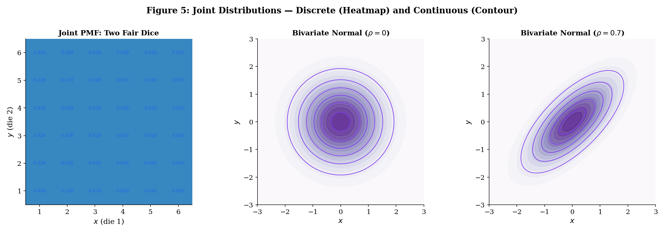
Roll two fair dice. Let = first die, = second die. The joint PMF is for . The marginal of is — as expected.
where . The joint PDF is
The parameter controls the correlation — the linear dependence between and . When , the joint factors as , and and are independent.
Explore joint distributions: toggle between discrete (two dice heatmap) and continuous (bivariate normal contours). Slide and watch the contours morph from circular (independent) to elliptical (dependent):
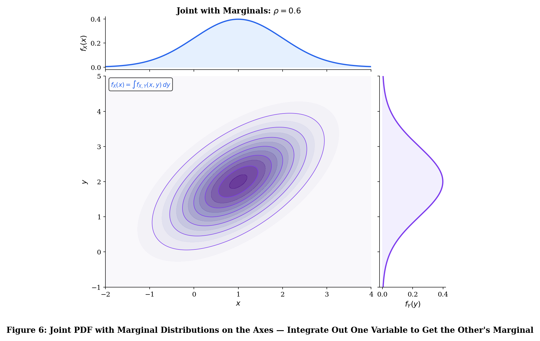
6. Marginal Distributions
For discrete , the marginal PMF of is
For continuous with joint PDF , the marginal PDF of is
In both cases, we “integrate out” (or “sum out”) the variable we don’t want. This connects directly to the law of total probability from Topic 2: the marginal is a weighted average over all possible values of the other variable.
The marginal distributions are uniquely determined by the joint distribution — sum over (discrete) or integrate out (continuous) the other variables.
Proof Marginals from the Joint (Theorem 2) [show]
For the discrete case:
Since are pairwise disjoint for different , countable additivity (Topic 1, Axiom 3) gives
Knowing and individually is not enough to reconstruct . The joint encodes the dependence structure between and — information lost when we marginalize. This is why “correlation does not imply causation” has a precise mathematical meaning: the marginals constrain the joint, but don’t determine it. Specifying the dependence structure is the job of copulas — see Multivariate Distributions.
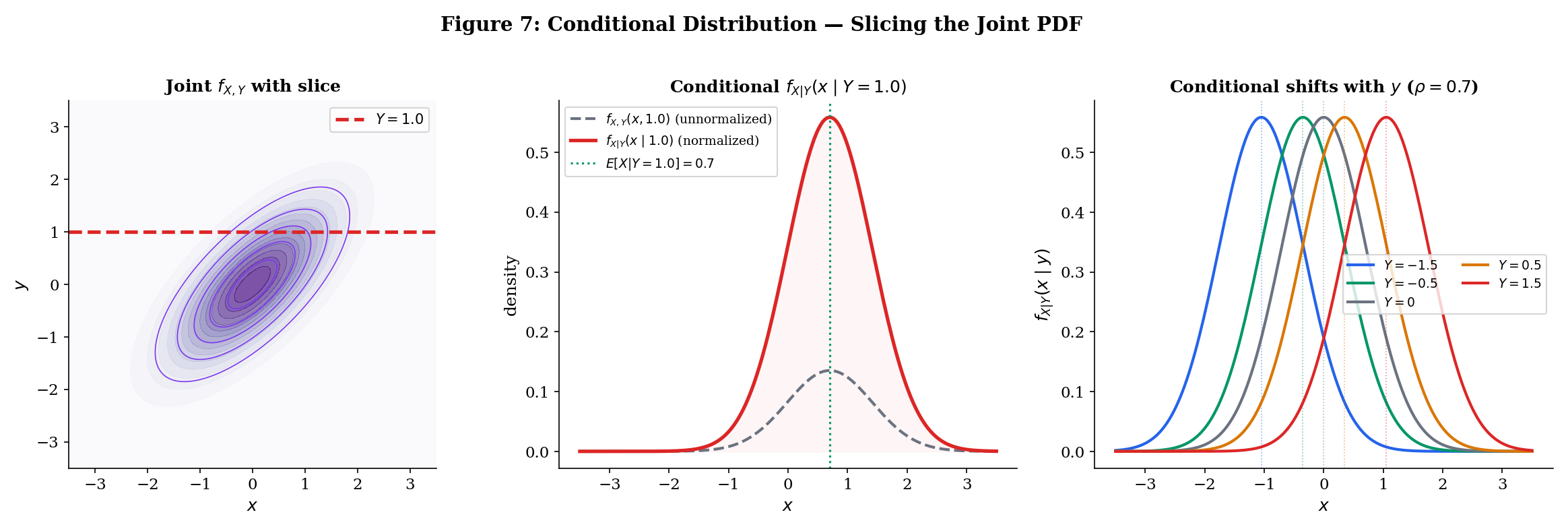
7. Conditional Distributions
Conditional distributions extend conditional probability (Topic 2) from events to random variables. Instead of "" for events, we ask "" — the distribution of given that takes a specific value.
For discrete with ,
This is exactly the definition of conditional probability (Topic 2, Definition 1) applied to the events and : .
For continuous with ,
This requires more care than the discrete case — since for continuous , we can’t directly condition on . The conditional PDF is defined as the limit . The formula above is the result of that limit.
The joint density factors as
This is the density version of the multiplication rule (Topic 2, Theorem 1). Rearranging gives the density version of Bayes’ theorem:
Proof Chain Rule for Densities (Theorem 3) [show]
Rearrange the definition to get
The symmetric factorization follows by exchanging the roles of and .
If are jointly normal with correlation , then is normal:
Two remarkable facts:
- The conditional mean is linear in : this is why linear regression works for jointly normal data.
- The conditional variance does not depend on — this is the homoscedasticity assumption.
8. Independence of Random Variables
Independence of random variables extends the concept of independence from events (Topic 2, Definitions 3–4) to distribution functions.
Random variables and are independent (written ) if for every pair of Borel sets ,
Equivalently, any of the following:
- CDF factorization: for all .
- PMF factorization (discrete): for all .
- PDF factorization (continuous): for all .
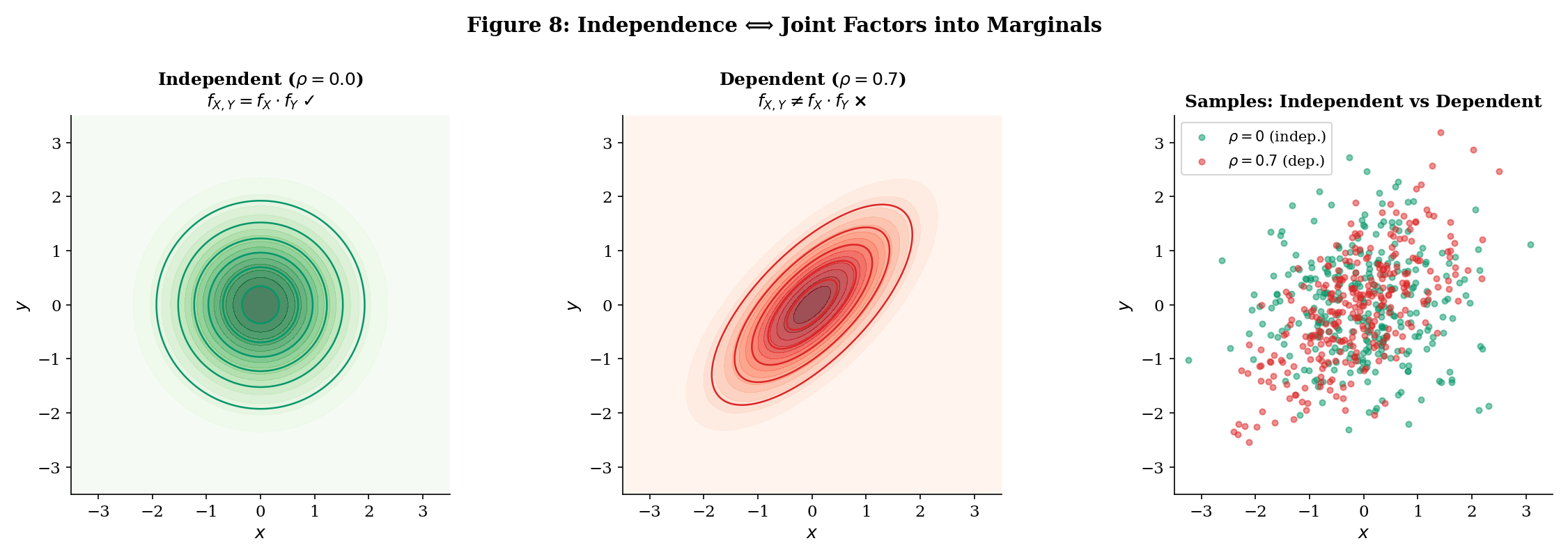
if and only if (continuous case) or (discrete case) for all .
Proof Independence ⟺ Joint Factors (Theorem 4) [show]
() Assume . Then for all :
Differentiating with respect to both and (using the multivariable chain rule):
() Assume . Then for any Borel sets :
The integral factors by Fubini’s theorem.
If , then — knowing tells you nothing new about .
Proof Independence ⟹ Conditional = Marginal (Theorem 5) [show]
This is the random variable version of the event independence criterion from Topic 2.
Let be bivariate normal. They are independent if and only if . When , knowing shifts the conditional mean of (by Example 9), so and are dependent. The contour plots make this visible: gives circular contours (factored density), gives elliptical contours (non-factored).
9. Transformations of Random Variables
If has a known distribution and for some function , what is the distribution of ? This arises constantly:
- If is a measurement, is a rescaled measurement.
- If , then — the inverse CDF transform.
- If is a model’s raw output, is the sigmoid-transformed probability.
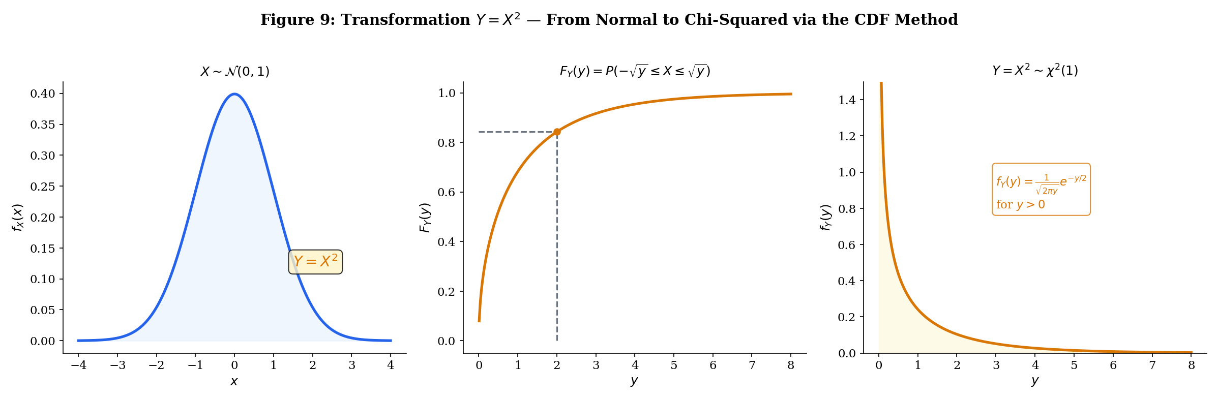
- If is a random variable, appears in the chi-squared distribution.
Let be a random variable with known CDF and let . Then
To find , solve the inequality for , then express the result in terms of .
Proof CDF Method (Theorem 6) [show]
This is the definition of CDF applied to . The content is in the method, not the proof.
Let with . Then
Differentiating: . If , the inequality flips and .
Application: If , then . Standardization is a linear transformation.
When is monotonic and differentiable, we get a direct formula for the PDF.
Let be a continuous random variable with PDF . Let where is strictly monotonic and differentiable with inverse . Then
The factor is the Jacobian — it accounts for how stretches or compresses intervals.
Proof Change of Variables for PDFs (Theorem 7) [show]
Assume is strictly increasing (the decreasing case is similar with a sign flip).
Differentiate using the chain rule:
Since is increasing, is also increasing, so .
For decreasing , the inequality flips: , and differentiating introduces a minus sign that the absolute value absorbs.
This proof uses the chain rule and substitution rule from formalCalculus: Change of Variables .
Let and (i.e., ). Then and . So
This is the lognormal distribution. It arises when the logarithm of a quantity is normally distributed — common for financial returns, biological measurements, and the distribution of weights in neural networks.
For a vector transformation where is a diffeomorphism, the change of variables formula becomes
where is the Jacobian matrix. This is the formula behind formalML: Normalizing Flows — a class of generative models that learn invertible transformations of simple distributions. Each flow layer applies this change of variables formula.
Pick a source distribution and a transformation to watch the CDF method produce the output distribution. Toggle Monte Carlo samples and watch the histogram converge:
Transformation: Y = X² — x² → χ²(1)
10. Expectation (Preview)
We close the mathematical content with a brief preview of the next topic. Once we have random variables and their distributions, the next natural question is: what is the “average” value?
The expectation (or expected value, or mean) of a random variable is
provided the sum or integral converges absolutely.
The expectation is the “center of mass” of the distribution — if you placed the PMF bars (or PDF curve) on a number line and balanced it on a fulcrum, the balance point is .
These concepts — along with variance, covariance, higher moments, and moment-generating functions — are the subject of Expectation, Variance & Moments. There we prove the linearity of expectation, derive the variance decomposition, establish the law of total expectation , and connect moments to the shapes of distributions.
11. Connections to ML
Feature Vectors as Random Vectors
Every dataset in ML is implicitly modeled as a sample from a random vector. A training example is a realization of the random vector where is the feature vector and is the target.
| ML Concept | Random Variable Formulation |
|---|---|
| Feature vector | Random vector |
| Training set | i.i.d. draws from |
| Class probabilities | PMF or conditional PMF |
| Regression target | Continuous with conditional density |
Generative vs. Discriminative: Joint vs. Conditional
The generative/discriminative distinction maps directly to joint vs. conditional distributions:
- Generative models learn the joint distribution — or equivalently, the class-conditional and prior . Examples: Gaussian Discriminant Analysis, naive Bayes, VAEs, diffusion models.
- Discriminative models learn the conditional distribution directly. Examples: logistic regression, neural networks, random forests.
From the joint, you can always get the conditional (via Bayes’ theorem from Topic 2). But generative models must model the full distribution — a harder problem in high dimensions.
Softmax Outputs as PMFs
A neural network classifier with softmax output computes for classes . This output is a PMF: for all , and by construction of softmax. The softmax function guarantees that the output satisfies the PMF axioms — making the network’s predictions interpretable as conditional probabilities.
Loss Functions as Transformations
The loss is a transformation of random variables. If and have known distributions, the distribution of determines the risk — and the change of variables formula (Theorem 7) is how we analyze it.
The Inverse CDF Transform
Let and let be any CDF with quantile function . Then has CDF .
Proof Universality of the Uniform (Theorem 8) [show]
since gives for .
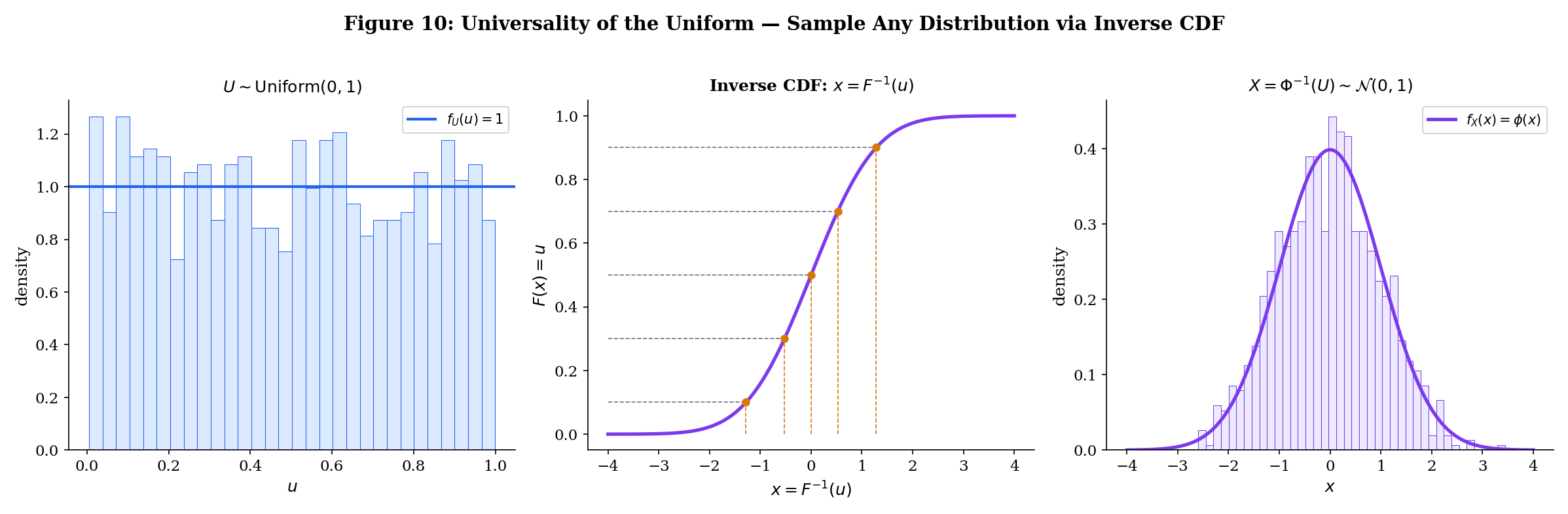
This is how you sample from any distribution using only uniform random numbers. It’s the foundation of Monte Carlo simulation and the basis of formalML: Normalizing Flows in generative modeling. The Fisher information metric that gives the space of distributions its geometry is developed in formalML: Information Geometry , and the KL divergence used in formalML: Variational Inference relies on the conditional PDF framework established here.
12. Summary
| Concept | Key Idea |
|---|---|
| Random variable | A measurable function mapping outcomes to numbers |
| PMF | Each value IS a probability (discrete) |
| NOT a probability; integrate for probability (continuous) | |
| CDF | The universal descriptor — works for all random variables |
| CDF properties | Non-decreasing, right-continuous, , |
| Joint distribution | Full description of two random variables together |
| Marginal | Integrate out / sum out the other variable |
| Conditional distribution | |
| Independence | iff |
| Transformation | : CDF method or change of variables with Jacobian |
| Inverse CDF transform | where generates |
What’s Next
Expectation, Variance & Moments answers: once we have distributions, what summaries do we compute? It defines expectation (), proves linearity, derives variance (), develops the law of total expectation (), and introduces moment-generating functions — the analytic tool that powers the proofs of the law of large numbers and the central limit theorem.
References
- Billingsley, P. (2012). Probability and Measure (Anniversary ed.). Wiley.
- Durrett, R. (2019). Probability: Theory and Examples (5th ed.). Cambridge University Press.
- Grimmett, G. & Stirzaker, D. (2020). Probability and Random Processes (4th ed.). Oxford University Press.
- Wasserman, L. (2004). All of Statistics. Springer.
- Casella, G. & Berger, R. L. (2002). Statistical Inference (2nd ed.). Duxbury.
- Bishop, C. M. (2006). Pattern Recognition and Machine Learning. Springer.
- Goodfellow, I., Bengio, Y. & Courville, A. (2016). Deep Learning. MIT Press.
- Kobyzev, I., Prince, S. J. D. & Brubaker, M. A. (2021). Normalizing Flows: An Introduction and Review of Current Methods. IEEE TPAMI, 43(11), 3964–3979.