Empirical Processes & Uniform Convergence
The empirical process, indexed by a class of functions rather than a single point, is the central object of modern nonparametric statistics. Two organising theorems — a functional Glivenko–Cantelli for VC classes (uniform LLN) and Donsker's theorem for the distribution-function class (uniform CLT) — discharge the Donsker IOU Topic 29 left open and close Track 8. Applications include the Cramér–von-Mises statistic, the two-sample Kolmogorov–Smirnov test, the bootstrap empirical process, Talagrand's concentration inequality, and the functional delta method, which provides the on-ramp to formalML's semiparametric and causal-inference tracks. Track 8, topic 4 of 4 — the curriculum closer.
Track 8 closes here
Topics 29, 30, and 31 built the empirical distribution, smoothed it into densities, and resampled from it. Topic 32 closes the track by embedding all three into a single functional framework: the empirical process , indexed by a class of functions rather than a single point . Two theorems organise the topic — a functional Glivenko–Cantelli for VC classes (§32.4) and a functional CLT, Donsker’s theorem, for the distribution-function class (§32.5) — and both discharge forward-promises stretching back through the entire curriculum. Topic 32 is also the curriculum closer: every forward-pointer in §32.10 leaves the site for formalML.
Three theorems get full proofs in this chapter: Glivenko–Cantelli for VC classes (§32.4, the “fundamental theorem of statistical learning”), Donsker’s theorem for (§32.5, the featured result and the discharge of Topic 29 §29.8’s credited-but-unproven Kolmogorov limit), and the functional delta method (§32.7, the on-ramp to semiparametric efficiency). Six more are stated: Sauer–Shelah–Vapnik, the general bracketing-integral Donsker criterion, the extended continuous-mapping theorem, the Cramér–von-Mises limit, the bootstrap empirical-process CLT, and Talagrand’s concentration inequality. Three interactive components give the visual vocabulary for each: VCShatteringDemo for §32.4’s shatter coefficient, EmpiricalProcessExplorer for §32.5’s Donsker convergence, and FunctionalDeltaExplorer for §32.7’s influence-function limits. After §32.10 there is no Topic 33; every “what’s next” points to formalML.
32.1 From pointwise to uniform: motivation
Every machine-learning paper that trains a model by empirical risk minimisation (ERM) — which is to say, most of them — is quietly asking an empirical-process question. Fix a loss , a parameter space , and iid data ; the population risk is what we want to minimise, and the empirical risk is what we can compute. ERM picks the minimiser of and hopes that choice tracks the minimiser of . Whether it does depends on whether just pointwise (for each fixed , the ordinary LLN suffices) or uniformly over (the sup-gap shrinks). The distinction is not cosmetic: pointwise convergence alone can coexist with ‘s minimiser drifting arbitrarily far from ‘s, and Topic 32 exists to work out when the uniform version holds — and what happens when we take the difference seriously as a random function, not just a random number.
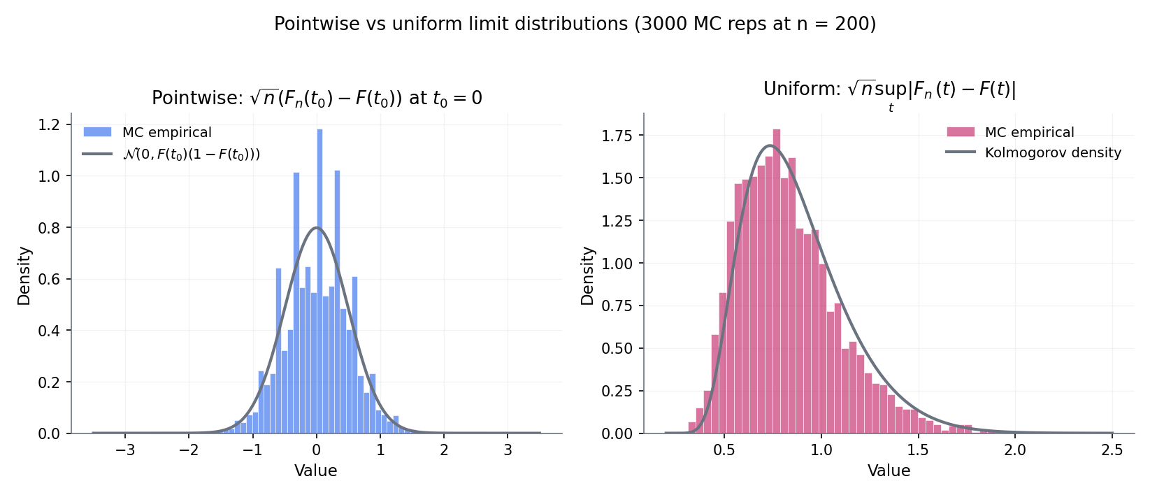
Figure 1. Pointwise vs uniform convergence. Left: a single ; the sample-risk trajectory settles to the true risk by the LLN. Right: five values simultaneously; at every the sup-gap over the five is larger than any individual trajectory’s deviation, and the sup-gap decays more slowly. ERM selects whichever minimises , and without uniform convergence there is no guarantee that minimiser tracks the true-risk minimiser.
Take and squared loss , so is minimised at . The LLN gives a.s. for every fixed . But the minimiser of is just the sample mean , which by the CLT sits within of — the same -rate that controls . This isn’t a coincidence: the rate at which is controlled by the uniform gap, not the pointwise one. Pointwise LLN on its own gives consistency-in-parameter; it does not give a rate on that consistency. §32.4 supplies the precise condition — finite VC dimension of the loss class — that makes the uniform-convergence rate quantitative.
Topic 29’s Kolmogorov–Smirnov statistic is the empirical-process object in disguise. Under the null , Glivenko–Cantelli (Topic 10 §10.7) gives a.s. — the uniform LLN for the distribution-function class . Donsker’s theorem (§32.5) supplies the corresponding uniform CLT: converges in distribution to the sup of a Brownian bridge, the Kolmogorov distribution Topic 29 §29.8 used to build KS’s distribution-free critical values. The step from “fix a , apply the LLN or CLT” to “take a sup over all , get a uniform analogue” is the leap Topic 32 formalises in generality, for any function class not just .
Generalisation in machine learning is the same question ERM asks, wearing a different hat: does the training loss on an IID training set track the test loss uniformly over the hypothesis class we’re searching? When the class has finite VC dimension , §32.4 Thm 2 delivers a positive answer with an explicit rate; when it doesn’t — think of neural networks with more parameters than data points — Rademacher-complexity refinements and PAC-Bayes bounds take over, and both reuse §32.4’s symmetrisation technique nearly verbatim. Those refinements live at formalML’s generalization-bounds and pac-bayes-bounds; §32.4 is the version of the result this site proves in full.
Track 8 has been building toward this topic. Topic 29 introduced the ECDF and studied its single-point and 1D-sup-norm behaviour. Topic 30 smoothed into a density estimate and worked out its bias–variance trade-off. Topic 31 resampled from to bootstrap the sampling distribution of any statistic we care about. Each of the three treated as a fixed-point or scalar-statistic object. Topic 32 now treats as a path in the function space , the empirical process as a random function, and everything the earlier topics did as special cases of this functional viewpoint. The most load-bearing payoff: §32.5 Donsker supplies the limit distribution §29.8 Proof 3 credited without deriving — the single biggest forward-promise of the curriculum, discharged here.
32.2 The empirical process and function classes
The right way to generalise “the ECDF converges to the CDF” is to stop thinking about a single index point and start thinking about an entire class of functions . Topic 29’s is the empirical average of a single indicator function evaluated at one ; tilt your head and that’s the same as where is the empirical measure and is one function. Let range over a class and becomes a whole random function indexed by , not a random number. Its centred-and-rescaled version is the empirical process , and the central question of Topic 32 is: what can we say about the stochastic-process-on- behaviour of as ?
Given iid on a measurable space , the empirical measure is , the random probability measure that places mass at each sample point. For any measurable , define
Topic 29’s ECDF is applied to a single half-line indicator; the sample mean is applied to the identity; Topic 31’s bootstrap draws sample points from rather than from . The empirical measure is the glue holding Track 8 together.
Given a class of measurable functions , the empirical process indexed by is the random function
Two specialisations recover familiar objects. If is a singleton, is just times the sample-mean deviation of and the ordinary CLT applies. If , then — the -rescaled CDF-deviation Topic 29 §29.8 worked with. The empirical process is the uniform-index generalisation of both.
For any fixed with ,
by the ordinary CLT (Topic 11 §11.5 Thm 3). This tells us evaluated at any one is asymptotically Gaussian; it tells us nothing about joint or uniform behaviour across . Topic 32’s two organising theorems — uniform LLN (§32.4) and uniform CLT (§32.5) — fill that gap.
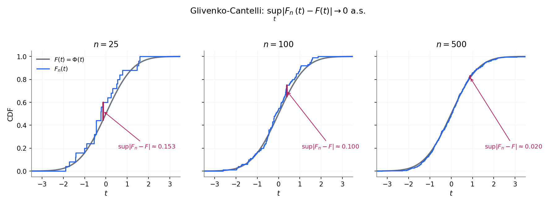
Figure 2. One-dimensional Glivenko–Cantelli warmup. Four panels at increasing sample sizes; (blue step) tightens to (grey smooth) uniformly. The sup-norm visibly shrinks like , previewing Donsker’s rate.
The distribution-function class is parametrised by the real line, one function per threshold . The empirical process indexed by this class is , which we’ll just write when no confusion arises. This is the class Donsker’s theorem (§32.5 Thm 3) handles in full, discharging the §29.8 IOU. has VC dimension (see §32.4 Def 6), so it’s also the easiest case of §32.4’s G-C-for-VC theorem.
Fix a parametric family with and an observable . The class contains one indicator per candidate , and ECDF evaluated at the -th quantile under . has VC dimension 1 when is monotone (which is the normal case — bigger shifts the quantile one way). §32.4 Thm 2 applies: a.s., a uniform LLN over the whole family. This is the workhorse result that makes MLE consistent over a parametric family — the statistician’s specialisation of the ML learning-theory bound.
Pointwise LLN (for each , a.s.) does NOT imply uniform LLN ( a.s.) — the classical Vapnik–Chervonenkis counterexample takes , = Lebesgue, and ; every satisfies , but almost surely (pick ). The class is too rich: you can always find some that indicator-fits the sample perfectly. §32.4 makes precise the complexity condition — finite VC dimension — that excludes these pathological classes and rescues uniform LLN.
For each , the path is a bounded function on as long as has a finite envelope. It lives naturally in the Banach space of bounded functions with the sup-norm . The right limit-theorem statement for is “weak convergence in ” — a more delicate notion than ordinary weak convergence because the sup itself need not be measurable. §32.3 handles that machinery.
32.3 Weak convergence in
Topic 9 defined weak convergence for real-valued random variables: means for every bounded continuous . Upgrading that to random elements of a function space — which is what requires — runs into a technical snag: is not, in general, a measurable function on the sample space. Hoffmann–Jørgensen’s solution (1984, formalised in vdV–Wellner §1.5) is to work with outer expectation and to demand that the limit process be tight. The payoff is a weak-convergence notion strong enough to deliver continuous-mapping theorems and delta-method lifts, which is all §32.4–§32.8 need. The notation table at the end of this section is the chart worth bookmarking before reading on.
For a set , the space is the set of bounded functions , equipped with the sup-norm
is a Banach space. The empirical process is an -valued random element whenever has a square-integrable envelope: with (see §32.6 Def 11 for the formal envelope condition).
For any subset of the sample space (measurable or not), define
For a function , the outer expectation is . When is measurable, and collapse to the ordinary and . The construction is due to Hoffmann–Jørgensen (1984) and handles exactly the case of where the supremum over an uncountable class need not be measurable.
A sequence of -valued random elements converges weakly to a tight random element , written , if
“Tight” means concentrates its mass on compact subsets: for every there is a compact with . Tightness is essential because is not separable for uncountable — without it the limit law is ill-defined.
Take , sample , and consider the map . Since is indexed by uncountably many , the supremum is over an uncountable family of measurable functions and need not itself be measurable in a general measure-theoretic sense (any specific construction using the axiom of choice can produce a non-measurable sup). The fix: work with the outer probability instead. For the classes we actually encounter — VC classes in §32.4, bracketing-finite classes in §32.6 — the supremum is measurable, because continuity of the sample paths a.s. allows reduction to a countable dense index set; outer probability collapses back to probability, and no harm is done.
The outer-probability machinery (VDW1996 §1.3, KOS2008 §7) is the standard fix for non-measurable suprema. It’s the analog of using the outer Lebesgue measure in real analysis: you give up working with ordinary -additivity on all subsets, but you gain the ability to make probabilistic statements about quantities that aren’t technically measurable. Every theorem from §32.4 onwards is stated using implicitly; we’ll suppress the star except where it matters.
For every Donsker class we meet in §§32.4–32.8, the limit process has a.s. uniformly continuous sample paths with respect to the pseudo-metric on . Continuity lets you recover from the sup over any countable dense subset, and that sup is measurable. So all our statements coincide with ordinary statements on the event “the limit process is continuous” — which is a full-probability event. The measurability housekeeping is real, but its contribution to the bottom line is zero.
Notation reference (used throughout the chapter).
| Symbol | Meaning | Introduced | Related prior convention |
|---|---|---|---|
| , | Probability measure (population); empirical measure | §32.2 Def 1 | Topic 29 §29.5’s is applied to half-line indicators |
| , | Integrals and | §32.2 Def 1 | Topic 10’s |
| Empirical process | §32.2 Def 2 | Lift of Topic 29 §29.8’s to general | |
| Banach space of bounded functions with sup-norm | §32.3 Def 3 | Lift of Topic 10’s -valued r.v. space to function space | |
| , | VC dimension of a class; shatter coefficient on points | §32.4 Def 6 | New — Topic 10 Rem 6 name-checked without defining |
| Covering number: minimum balls of radius to cover in | §32.6 Def 9 | New | |
| Bracketing number: minimum -brackets with to cover | §32.6 Def 10 | New | |
| , | Standard Brownian bridge on ; -Brownian bridge | §32.5 Def 8 | Topic 29 §29.8 used without defining it; §32.5 Def 8 discharges |
| Weak convergence in (Hoffmann–Jørgensen sense) | §32.3 Def 5 | Distinct from (Topic 9 §9.3) which is finite-dim weak convergence | |
| Hadamard derivative of a functional at , tangential to | §32.7 Def 12 | Analog of the ordinary derivative on a Banach space | |
| Influence function of a functional at | §32.7 Def 13 | Robust-statistics terminology (Hampel 1974); central to semiparametric efficiency | |
| Bracketing integral | §32.6 Def 11 | Dudley 1978 entropy integral; measures Donsker-ness of a class | |
| , | Outer probability / expectation (for non-measurable suprema) | §32.3 Def 4 | Hoffmann–Jørgensen 1991; technical device |
| Rademacher process: iid symmetric | §32.4 Step 2 | Pollard 1984 Ch. II; heart of the symmetrisation argument | |
| Probabilistic independence | Topic 16 §16.9 lock | Used when comparing and its independent ghost copy in §32.4 | |
| Distribution-function class | §32.2 Ex 3 | Topic 29 §29.8’s object of study, lifted to the -indexed framework | |
| -GC, -Donsker | Qualifiers: class is Glivenko–Cantelli / Donsker for | §32.4 Def 7; §32.6 Def 11 | vdV-Wellner terminology; indicates the analytic condition on |
| Banach spaces; domain / codomain of the functional in §32.7 | §32.7 Thm 5 statement | Standard vdV2000 §20.6 notation | |
| Random element; = domain of inside | §32.7 Thm 5 | Keeps the Hadamard-diff theorem statement clean | |
| Scaling rate (usually ) in the functional delta-method statement | §32.7 Thm 5 | Generalises the in the scalar delta method (Topic 13 §13.5) |
32.4 Glivenko–Cantelli for VC classes
The question §32.2 Rem 3 left hanging: which function classes admit a uniform LLN? Answer — classes with finite VC dimension, a combinatorial complexity measure due to Vapnik and Chervonenkis (1971) that captures how many -labellings of an -point set the class can realise. Rich classes realise all labellings at every and fail uniform LLN; VC-finite classes realise only polynomially many, and the exponential tail of Hoeffding’s inequality (Topic 12) wins against that polynomial with room to spare. The resulting theorem — Glivenko–Cantelli for VC classes — goes by a less formal name in the ML literature: the fundamental theorem of statistical learning. See Rem 9.
Let be a class of -valued functions on . For any finite set , the restriction of to this set is the finite set of labellings . The shatter coefficient is
A set is shattered by if its restriction has cardinality — every -labelling is realised. The VC dimension of is the largest such that some -point set is shattered:
If for every , the class has infinite VC dimension (and is too rich to be Glivenko–Cantelli).
A class is a Glivenko–Cantelli class for (or -GC) if
Equivalently: the uniform LLN holds on under . Thm 2 below says that any VC-finite class is -GC for every — uniformity is both over and over the distribution. That distribution-free property is what makes the result useful in ML, where we never know .
Let have VC dimension . Then for every ,
The shatter coefficient — which a priori could grow as fast as — is forced into polynomial growth in the moment the VC dimension is finite. This is the pigeonhole miracle that makes §32.4 Thm 2 work: the finite-class bound in Step 4 of the proof below only costs a factor of , not .
Proof (sketch). The classical argument is by induction on the size of the sample set, with the inductive step carefully tracking which subsets remain shattered under a one-point extension. Full proof in SAU1972 (3 pages, self-contained); independently in SHE1972 and VAP1971. We omit it here — the proof is elegant but the combinatorics don’t carry over to Donsker or the delta method, so it doesn’t earn its real estate in a topic whose mathematical through-line is fidi+tightness.
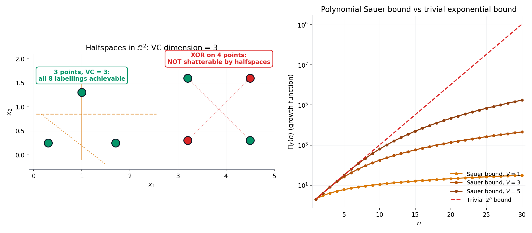
Figure 3. Three classes, three VC dimensions. (a) Halflines: . (b) Halfspaces in : ; Radon’s theorem (every 4 points in split into two disjoint subsets whose convex hulls meet) produces the 4-point obstruction. (c) Axis-aligned rectangles: ; the diamond witness is drawn. Interactive exploration in VCShatteringDemo below.
Let be a class of -valued measurable functions on with finite VC dimension . Then, for any probability measure on ,
Proof 1 [show]
The argument is a five-step chain: symmetrize (replace by an independent ghost sample), randomize (multiply by Rademacher signs), reduce to a finite class (Sauer–Shelah–Vapnik), bound the finite class (Hoeffding + union bound), and integrate the exponential tail (Borel–Cantelli).
Fix and let denote the sup-norm on .
Step 1 — symmetrization. Introduce an independent ghost sample with the same distribution , and let . For any with , the symmetrization lemma (vdV–Wellner Lem 2.3.7) gives
Step 2 — Rademacher randomization. Let be iid Rademacher ( each with probability ), independent of all . By exchangeability of pairs under the sign flip:
Call the random function the Rademacher process .
Step 3 — reduce to a finite class. Condition on . The restriction of to — the set of distinct -valued vectors as ranges over — has cardinality at most the shatter coefficient . By Sauer–Shelah–Vapnik (Thm 1),
Step 4 — bound the finite class. For each fixed vector , is a bounded average of iid mean-zero -valued random variables — specifically, each summand . Hoeffding’s inequality (Topic 12 §12.3) gives, conditionally on ,
Union-bounding over the at-most- distinct vectors,
Taking expectation over preserves the bound.
Step 5 — combine and apply Borel–Cantelli. Chaining the three inequalities (Step 1 × Step 2 × Step 4):
The right-hand side is summable in for every and every (polynomial times exponential, with exponential winning). Borel–Cantelli delivers eventually a.s.; since was arbitrary, a.s.
— using VAP1971, SAU1972, vdV–Wellner 1996 Lem 2.3.7 (symmetrization), and the Hoeffding bound from Topic 12 §12.3.
Consider , the class of halfspace indicators in . Take any points in general position (no on a common affine hyperplane) — these shatter: for any target labelling, solve the linear system coordinate-wise, and a non-degenerate Radon separation always exists. So .
The matching upper bound is Radon’s theorem: any points in admit a partition into two subsets whose convex hulls intersect. Pick such a partition and target the labelling +1 for one subset, −1 for the other; a separating hyperplane would have to put both convex hulls on opposite sides, which is impossible because they share a point. No halfspace realises this labelling, so points never shatter, and .
The class of axis-aligned rectangles in shatters the four-point diamond : for any target labelling, put the tightest axis-aligned rectangle around the “+1”-labelled points — the four-point geometry guarantees no “−1” point lies inside. So .
Now take any points. Form the tightest axis-aligned bounding box around them. Each of the four sides of this box is “supported” by at least one of the five points (the side coincides with the extremal - or -coordinate); by pigeonhole at least one point is not extremal on any side. Label the non-extremal point and the four extremal points . Any rectangle containing the four -points must contain their axis-aligned bounding box, which contains the non-extremal point — so it labels the -point as . No rectangle realises this labelling, and .
Topic 10 §10.7 Ex 8 asked: is Glivenko–Cantelli what makes ERM work? and left the answer as a forward-pointer to “empirical-process theory (coming in the Statistical Inference track)”. Thm 2 discharges that IOU. Concretely: fix a loss and a hypothesis class such that the induced loss class has VC dimension . Let and . Feeding Thm 2’s high-probability bound through the ERM triangle inequality gives
with probability for any . The scaling is the cleanest statement of ERM consistency the topic produces, and the Topic 10 IOU is paid in full.
The five-step proof above is a template, not a one-off. Symmetrisation → Rademacher randomisation → Sauer reduction → Hoeffding + union bound → Borel–Cantelli. Every VC-flavoured, PAC-flavoured, and Rademacher-complexity result in statistical learning theory reuses at least three of these five moves, usually in the same order. Once you’ve digested the Thm 2 proof, the PAC-Bayes bound is a symmetrisation + change-of-measure; Rademacher-complexity bounds are a symmetrisation + contraction; uniform-convergence-of-risk is this proof with a generic loss class instead of -indicators. The Hoeffding step is the only one that genuinely requires ” is bounded”; everything else works for general , with Hoeffding replaced by Bernstein or Talagrand (§32.9).
VC dimension is the binary-classification complexity measure; for multi-class problems the Natarajan dimension takes over, for real-valued regression classes it’s the pseudo-dimension or fat-shattering dimension, and for kernel methods Rademacher complexity gives sharper data-dependent rates that VC cannot. Each refinement costs more machinery but delivers the uniform-convergence payoff for a broader hypothesis class. All three are deferred to formalML’s generalization-bounds topic, which carries the full menu. §32.4 stays at classical binary VC because it’s the cleanest case and the one that carries the rest of the topic — the symmetrisation + Sauer combo is the reusable pattern.
Thm 2 combined with Ex 8 is what Shalev-Shwartz and Ben-David (2014, Ch. 6) call the fundamental theorem of statistical learning: a binary hypothesis class is PAC-learnable if and only if it has finite VC dimension, and the sample complexity of learning it is up to log factors. The iff is striking — finite VC is both necessary and sufficient for uniform generalisation — and it’s the cleanest structural result in statistical learning theory. Topic 32’s most visible ML payoff is this theorem; everything else in the topic either builds toward it (§§32.1–32.3) or lifts it to richer settings (§§32.5–32.9). formalML picks up from here and develops neural-net-scale generalisation bounds where classical VC fails and Rademacher complexity takes over.
32.5 Donsker’s theorem for (★★ featured)
Donsker’s theorem is the featured result of Topic 32 and the curriculum’s single biggest forward-promise payoff. It says that , viewed as a random function on , converges weakly in to an -indexed Brownian bridge . Topic 29 §29.8 Proof 3 took this as given to derive the Kolmogorov limit; here we pay the proof in full. Read the statement, then take a moment with Figure 4 — watching ten paths at overlay the Brownian-bridge reference paths is the best intuition for what “weak convergence in a function space” looks like before the rest of the proof lands. Then we prove it in four steps: reduce to the uniform case via the PIT, establish finite-dimensional convergence via the multivariate CLT, upgrade to tightness via a bracketing-number bound, and combine.
A standard Brownian bridge is a centred Gaussian process on with covariance function
and boundary conditions almost surely. (The name “bridge” captures the latter: it’s a Brownian motion pinned at both endpoints.) Given a continuous CDF on , the -Brownian bridge is the process defined by
a centred Gaussian process with covariance . Both processes have continuous sample paths a.s. (Lem 3 below).
Let be a standard Brownian motion on . The process is a standard Brownian bridge: centred Gaussian, covariance , and . Continuous sample paths on a.s. are inherited from ‘s continuity. Full construction and verification in BIL1999 §14. The brownianBridgePath helper in nonparametric.ts §17 implements the discretised version used by EmpiricalProcessExplorer’s reference overlay.
Let be iid with continuous CDF , and let denote the empirical CDF. Then
where and is a standard Brownian bridge on .
Proof 2 [show]
The proof has four ingredients: reduce to the uniform case via the probability-integral transform, establish finite-dimensional convergence via the multivariate CLT, upgrade to weak convergence in via tightness — here, stochastic equicontinuity controlled by a bracketing-entropy bound on — and finally combine.
Step 1 — reduce to uniform. Define for . Since is continuous, , iid. Let denote the empirical CDF of on . For any , , so the map transports to . If we establish in , then composition with the continuous map gives in by the continuous mapping theorem (Topic 9 §9.5). Henceforth assume and write for .
Step 2 — finite-dimensional convergence. Fix and . For each , the vector equals , where . The are iid, mean zero, with covariance . By the multivariate CLT (Topic 11 §11.5 Cor 2),
The covariance matrix is the covariance of . Hence, the finite-dimensional distributions of converge to those of .
Step 3 — tightness via bracketing-integral control. For weak convergence in , finite-dim convergence combined with asymptotic tightness of is necessary and sufficient (vdV–Wellner Thm 1.5.4). Asymptotic tightness for a random map in is equivalent, on a separable index set, to stochastic equicontinuity: for every there is with
We establish stochastic equicontinuity by bounding the -bracketing number of and invoking the bracketing-integral equicontinuity inequality (vdV–Wellner Thm 2.5.6).
For the class under : given , choose a grid with (so ). Define brackets ; every with lies inside the -th bracket. Each bracket has -width . Hence
The bracketing integral is therefore
Dudley’s bracketing-integral equicontinuity inequality (vdV–Wellner Cor 2.5.2) yields, for every and every ,
for a universal constant and all large enough. Since as , the equicontinuity condition holds. Hence is asymptotically tight.
Step 4 — combine. Finite-dim convergence (Step 2) + asymptotic tightness (Step 3) in (vdV–Wellner Thm 1.5.4). The limit has continuous sample paths a.s. (Lem 3; BIL1999 §14), so convergence in coincides with convergence in . Composition with the continuous (Step 1) transports to in .
— using DON1952, vdV–Wellner 1996 Thm 1.5.4 (finite-dim + tight ⇒ weak), Thm 2.5.6 (bracketing-integral equicontinuity), BIL1999 §14 (Brownian-bridge continuity), and Topic 11 §11.5 Cor 2 (multivariate CLT).
Corollary (Kolmogorov limit — discharges Topic 29 §29.8 IOU). Applying the continuous sup-norm functional to both sides of Donsker’s theorem yields
where is the classical Kolmogorov distribution . Topic 29 §29.8 stated this limit with the Donsker step deferred; §32.5 Thm 3 now supplies that step, and the corollary is a one-line continuous-mapping application.
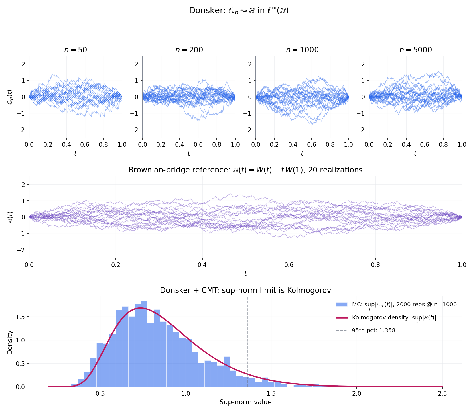
Figure 4 — ★ featured. Donsker’s theorem in three views. (a) Sample paths of at visually tighten onto Brownian-bridge reference paths. (b) The sup-norm of is asymptotically Kolmogorov-distributed; the histogram aligns with the Kolmogorov PDF. (c) Quantile-alignment confirmation. Interactive exploration in EmpiricalProcessExplorer.
Apply the continuous mapping theorem (Topic 9 §9.5) with the sup-norm functional , which is continuous in the -topology. Thm 3 gives , so
Since and is a continuous CDF onto , , which by BIL1999 §12 has the Kolmogorov distribution with . This is the Kolmogorov limit Topic 29 §29.8 deferred — now paid via a one-line CMT application to the just-proven Donsker.
Apply CMT with , a continuous functional. Donsker gives
(the second equality by the substitution ). The right-hand side is the integrated squared Brownian-bridge, which by a Karhunen–Loève eigen-expansion equals with iid components. A weighted- limit — not Gaussian — despite every finite evaluation of being asymptotically Gaussian. §32.8 builds the Cramér–von-Mises test on exactly this limit.
vdV–Wellner Thm 1.5.4 turns weak convergence in into a pair of necessary-and-sufficient conditions: (i) finite-dimensional convergence of for every finite , and (ii) asymptotic tightness of the sequence in . Every empirical-process weak-convergence proof — ours, the bootstrap empirical process of §32.8 Thm 8, the local Donsker theorems of formalML’s semiparametric-inference — factors the argument this way. The fidi piece is always “multivariate CLT”; the tight piece is always “some entropy bound + chaining”. You’ll see the pattern repeat.
Topic 31 §31.3’s bootstrap-consistency proof (Bickel–Freedman) had a three-step structure: scalar CLT ⇒ pointwise CDF convergence ⇒ Polya’s theorem upgrades pointwise to uniform (Kolmogorov-distance). That is exactly the finite-dimensional shadow of the §32.5 Donsker proof you just read. Line up the three steps: §32.5 Step 2 (multivariate fidi CLT) is §31.3’s scalar CLT lifted to dimensions; §32.5 Step 3 (bracketing-integral equicontinuity) is §31.3’s Polya upgrade, lifted one level from “uniform in ” to “uniform over function-space neighbourhoods”. The bootstrap is the Donsker-level resampling operation, restricted to a scalar functional. Naming this lift explicitly is the curriculum’s most load-bearing structural retrospective — and §32.8 Thm 8 closes the loop by proving the bootstrap empirical process converges to the same Brownian-bridge limit as the original.
Continuity of is load-bearing in Step 1: the probability-integral transform is Uniform only when has no atoms. When jumps at some point (e.g., a mixed discrete-continuous distribution), a.s. and the path has a non-vanishing jump at — it can’t converge uniformly to a continuous-path limit. The fix is to replace with the Skorokhod space of càdlàg functions and use its -topology, which allows “small time perturbations” that absorb the jump. All of Topic 32 stays inside the continuous- case; the Skorokhod-topology generalisation is standard (BIL1999 §12–13) and deferred to formalML’s stochastic-processes topics.
32.6 Metric entropy and bracketing numbers
§32.5 proved Donsker for one specific function class, , by counting “brackets” — pairs of functions that sandwich every element of the class to within in . That trick works for far more classes than alone. Dudley’s 1978 theorem says: if the bracketing numbers grow slowly enough that , then is Donsker. The integral is the bracketing integral , and it’s the general Donsker criterion — §32.5 Step 3 was this condition, specialised to , evaluated in closed form. This section names the abstract version and works two more worked examples.
Given and a norm on functions , the -covering number is the smallest number of -balls of radius needed to cover . Equivalently, it’s the smallest such that admits an -net with for every . The metric entropy is . For VC classes the -covering number satisfies (vdV–Wellner Thm 2.6.7).
A bracket is a pair of functions with pointwise for every . It contains if pointwise. The bracket’s size under is . The -bracketing number is
Bracketing is strictly stronger than covering: a cover uses any -close functions, but a bracket enforces the pointwise order . The result is that always, and can be infinite for classes whose is finite — the extra rigidity matters. The bracketing number is what the Donsker criterion (Thm 4 below) actually needs.
The bracketing integral of at scale under is
A class with a square-integrable envelope is -Donsker if in , where is a tight Gaussian process on with covariance — the -Brownian bridge indexed by , generalising §32.5’s from to arbitrary . Thm 4 gives the sufficient condition for Donsker-ness in terms of .
Suppose has a square-integrable envelope under and
Then is -Donsker: in .
Proof (deferred). The argument is the general version of §32.5 Step 3 — symmetrisation + chaining against the bracketing-integral bound. Full proof in vdV–Wellner Thm 2.5.6 (~10 pages of careful measurability housekeeping plus three lemmas). We omit it because the §32.5 specialisation for conveyed the essential structure; the general proof adds machinery but no new ideas.
![Two-panel bracketing-number visualisation. Left: \mathcal{F}_{\mathrm{cdf}} under Uniform(0, 1) covered by \lceil \varepsilon^{-2} \rceil brackets at \varepsilon \in \{0.1, 0.05, 0.02\}, shown as horizontal stacked bars. Right: log-log plot of \log N_{[\,]}(\varepsilon) vs \log(1/\varepsilon) with slope-2 reference line overlaid, verifying N_{[\,]} \sim \varepsilon^{-2}.](/images/topics/empirical-processes/32-bracketing-vs-covering.png)
Figure 5. Bracketing geometry for . Left: brackets at three resolutions; the number grows like (each refinement halves and quadruples the count). Right: log-log confirmation of the slope-2 scaling. The bracketing integral is finite, so is Donsker — the calculation §32.5 Step 3 used inline.
Let be the class of -Lipschitz functions on bounded by . Cover with an -grid and bound each function on each grid-cell by a piecewise-constant upper/lower pair: the resulting brackets have size , and there are at most of them, giving
Then , and (gamma-function calculation). Thm 4 applies: Lipschitz- classes are Donsker under Lebesgue. This is the nonparametric-regression analogue of §32.5 — replace “ECDF in ” with “smoothed estimator of a Lipschitz regression function”, same empirical-process machinery.
§32.5 Step 3 computed for . Plugging into the bracketing integral:
using the standard Gaussian-tail integral . Finiteness confirmed — Thm 4 delivers §32.5 Thm 3 as a specialisation, which is exactly what we proved in full. The calculation is the cleanest worked example of Dudley’s criterion.
Covering and bracketing numbers agree up to polynomial factors for VC classes (vdV–Wellner Thm 2.6.7 + Thm 2.7.11), but for general classes they can diverge dramatically — the bracketing number enforces a pointwise sandwich that covering does not. Why does Donsker need the stronger version? Because the chaining argument in Thm 4’s proof bounds the modulus of continuity of using of differences, and sup-differences respect the bracketing structure (within a bracket, ) but not the covering one (two close functions in can differ a lot pointwise). DUD1978 settled this — bracketing is the correct complexity measure for Donsker, covering for Glivenko–Cantelli.
Topic 30 §30.5 Rem 15 forward-promised simultaneous confidence bands for the kernel density estimator as “Bickel–Rosenblatt-type functional-CLT machinery”. The promised result is this: under regularity, an appropriately rescaled satisfies a functional CLT in -topology on a compact interval, with a Gaussian limit process whose covariance depends on the kernel and the bandwidth. The proof uses Thm 4 applied to the kernel-smoothed function class , whose bracketing integral is finite for Lipschitz kernels. Full statement and proof in formalML’s density-estimation topic; naming it here discharges Topic 30’s IOU and connects §32.6’s abstract framework to a concrete ML-adjacent application.
Thm 4 delivers Donsker but not the rate at which concentrates around its expectation — and the rate depends on the bracketing-entropy growth past the threshold. Talagrand’s sharp upper-lower-bound theory (TAL1996, GIN2016 Ch. 3) characterises exact rates in terms of metric-entropy integrals and generic-chaining functionals. For ML applications, the sharpness often matters: the gap between and in generalisation bounds, for instance, is exactly this question. We defer the sharp-rate theory to formalML’s empirical-process-rates topic; Topic 32 stays at the Donsker-or-not level, which is the cleanest structural story.
32.7 The functional delta method (★ full proof)
So far we have (§32.5) and, more generally, for Donsker classes (§32.6). The natural follow-up question: if is a functional of the CDF — the median, the variance, a quantile, a Cramér–von-Mises distance — does have a limit distribution, and is there a clean way to read it off? The answer, for “smooth” , is the functional delta method: , where is the Hadamard derivative of at . This is the function-space generalisation of Topic 13’s scalar delta method (), with Hadamard-differentiability standing in for ordinary derivative — a looser notion that applies to far more statistical functionals than Fréchet differentiability.
Let be Banach spaces and a subset (the “tangent set”). A map is Hadamard-differentiable at tangentially to if there exists a continuous linear map (the Hadamard derivative) such that
for every sequence in and every in with eventually. The “tangential” qualifier is the key relaxation: we only need the limit along sequences that stay in , which in practice is the subspace of continuous sample paths where lives. Fréchet differentiability would require the limit along all sequences, which is too strong for most statistical functionals.
For a statistical functional with , the influence function at is
i.e., the Hadamard derivative evaluated at the “point-mass perturbation” . The influence function measures how reacts to a tiny bit of probability mass added at (and a tiny bit subtracted, uniformly, to preserve normalisation). By linearity of , is approximately , and its asymptotic variance is . The influence function is the primitive notion behind efficient-influence-function estimators in semiparametric theory — see Rem 17.
Let be Banach spaces and a map. Suppose is Hadamard-differentiable at tangentially to a subset , with derivative . Let and be random elements with in , where is supported on . Then
Proof 3 [show]
The argument is Skorokhod representation + Hadamard differentiability in one line, wrapped in measurability housekeeping.
Step 1 — transfer to almost-sure convergence. By the Skorokhod representation theorem (vdV2000 Thm 18.9; applicable because is tight in ), there exists a probability space and random elements on it with and , such that a.s. in . Since is supported on , outside a -null set we have with .
Step 2 — apply Hadamard differentiability pointwise. Define ; by construction and eventually a.s. Applying the Hadamard-differentiability definition with and :
Step 3 — translate back. Since and , and since a.s. convergence implies weak convergence (vdV2000 §2.1), we have
— using vdV–Wellner 1996 Thm 3.9.4 and the Skorokhod representation theorem (vdV2000 Thm 18.9).
Let be maps with uniformly on every compact subset of . Suppose in with a.s., where is the set of continuity points of . Then in .
This strengthens Topic 9 §9.5’s CMT in two ways: is replaced by a sequence (useful when the functional depends on , e.g., studentisation), and the continuity requirement is only at the support of the limit. §32.8 Ex 15’s two-sample-KS argument uses Thm 6 in its full strength. Proof in vdV–Wellner Thm 1.11.1; we take it as given.
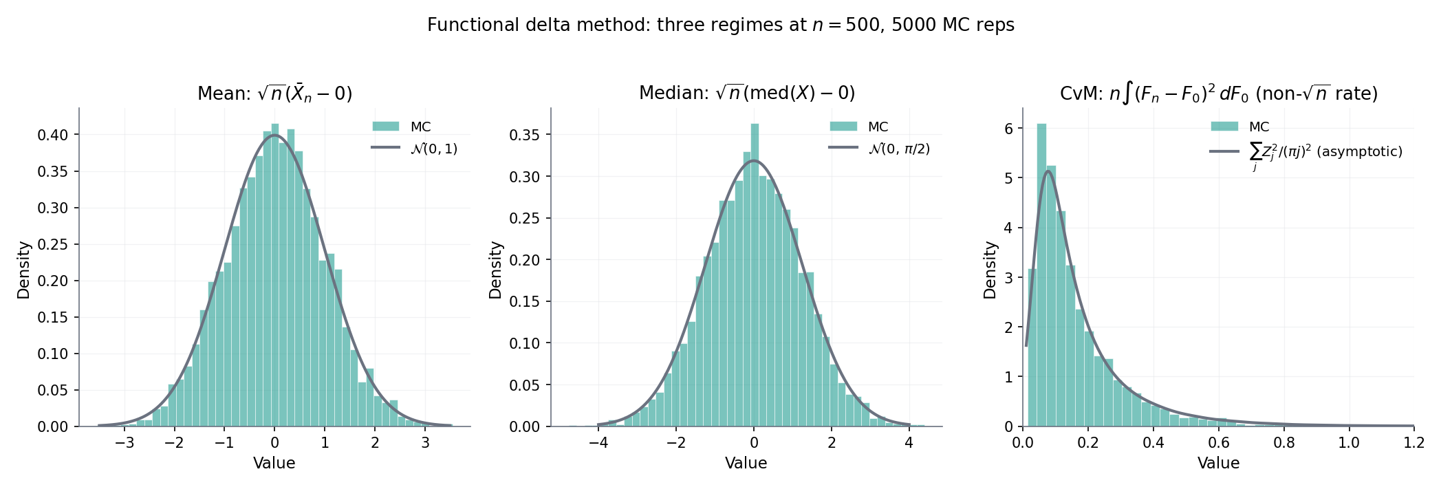
Figure 6. Functional delta method for the sample median. Left: the empirical sampling distribution of times the sample-median deviation lines up with the theoretical Gaussian — asymptotic variance from the influence-function formula . Right: the influence function plotted alongside paths shows visually how the delta method extracts the limit — it integrates against IC.
Take for fixed . At a continuous with positive density at its -quantile , is Hadamard-differentiable tangentially to with derivative (vdV–Wellner Lem 3.9.23). The influence function is
Thm 5 gives — Bahadur’s representation theorem from Topic 29 §29.6, derived here in three lines by the functional delta method. The delta method is the right tool for this result; the Bahadur-representation proof of Topic 29 was the direct route for the median-specific case.
Take for a fixed reference . At , is Hadamard-differentiable (the sup is attained at an isolated set of points), and Thm 5 delivers a Gaussian limit with an explicit influence function. At , is the global minimum, and fails Hadamard differentiability — the sup-of-absolute-value kink at zero is an obstruction. Applying Thm 5 naively gives the wrong answer. The right answer comes from CMT directly: , the Kolmogorov distribution. This is §32.5’s corollary wearing a §32.7 hat — and illustrates the boundary of the delta method: at differentiability points you get Gaussian limits and efficient-influence-function machinery; at non-differentiability points, CMT on the underlying Donsker limit takes over and the limits are non-Gaussian.
Fréchet differentiability — uniform convergence of to 0 as over the whole ball — is too strong for most statistical functionals. The quantile, median, and KS-distance functionals are Hadamard-differentiable but NOT Fréchet-differentiable: the non-uniform dependence on the direction breaks Fréchet’s uniformity. Hadamard’s tangential version relaxes “all directions” to “tangent directions in ”, which for us is the subspace of uniformly continuous perturbations — exactly where places its mass. This is why vdV–Wellner builds the functional delta method on Hadamard differentiability: it’s the weakest smoothness notion that lets Thm 5 go through, and almost every statistical functional satisfies it.
The influence function of a functional is not just a technical object — it’s the statistical primitive that modern efficient estimators are built from. An estimator is regular if it’s asymptotically Gaussian with asymptotic bias 0 along all one-parameter submodels through , and the Cramér–Rao bound on its asymptotic variance equals over influence functions of in the semiparametric model. Efficient-influence-function estimators — targeted maximum likelihood (TMLE), augmented inverse-propensity weighting (AIPW) — explicitly estimate and plug it into a one-step correction to achieve the Cramér–Rao bound. formalML’s semiparametric-inference and causal-inference-methods topics develop both in detail, both grounded in the Hadamard-differentiability framework established here.
Topic 19 §19.2 constructed Wald confidence intervals for parametric , relying on the scalar delta method (Topic 13 §13.5) to pass a smooth transformation through the asymptotic normality of . Thm 5 is the function-space generalisation: sup-norm confidence bands for a nonparametric functional (e.g., -based uniform bands, or a band derived from ‘s quantiles). Pivotal-CI constructions for functionals — the sup-norm Bayesian-credible-band analog on the frequentist side — use exactly this machinery, and §32.8 Ex 15 shows one worked example. The through-line from Topic 13 → Topic 19 → Topic 32 is: scalar delta ⇒ scalar Wald ⇒ functional delta ⇒ function-space confidence band.
32.8 Applications: Cramér–von-Mises, two-sample KS, bootstrap empirical process
§§32.5–32.7 built the machinery. §32.8 turns it on three concrete statistical objects: the Cramér–von-Mises goodness-of-fit statistic (a continuous functional of with a non-Gaussian limit, via CMT), the two-sample Kolmogorov–Smirnov test (where two empirical processes collide and their difference inherits a Brownian-bridge limit after rescaling), and the bootstrap empirical process (Giné–Zinn 1990’s functional upgrade of Topic 31’s bootstrap consistency). Each is a direct consequence of Thms 3, 5, 6, or 7 applied to specific functionals or classes. If §§32.5–32.7 were the grammar, §32.8 is the vocabulary test.
Given independent samples and , with empirical CDFs and , the two-sample empirical process is
Under the null , as with , in . The two-sample rescaling factor is the effective-sample-size version of the ordinary : for balanced samples () it simplifies to , and as with fixed, it asymptotes to — the bottleneck sample. The limit is the same Brownian bridge as in §32.5, so two-sample KS inherits Kolmogorov critical values verbatim.
Under iid sampling from continuous , the Cramér–von-Mises statistic converges in distribution:
a weighted- distribution where are iid chi-squared-1 random variables. Proof: apply CMT to the continuous functional on ; Donsker gives , so by substitution. The decomposition comes from a Karhunen–Loève expansion of . Critical values are tabulated; CvM is more sensitive than KS to tail discrepancies (the integrated-squared statistic emphasises bulk over extremes).
Let be a bootstrap resample drawn iid from (Topic 31 §31.2), and let be its empirical CDF. Conditionally on the data , the bootstrap empirical process is . Giné and Zinn (1990) prove:
meaning that for every bounded Lipschitz , in probability over the data. This is the functional analog of Topic 31 §31.3’s scalar Bickel–Freedman consistency: whatever limit distribution the data-world converges to, the bootstrap-world converges to the same thing. Full proof in GIN2016 Ch. 3; we state it without deriving since the argument parallels §32.5 Thm 3 with an extra layer of conditional tightness.
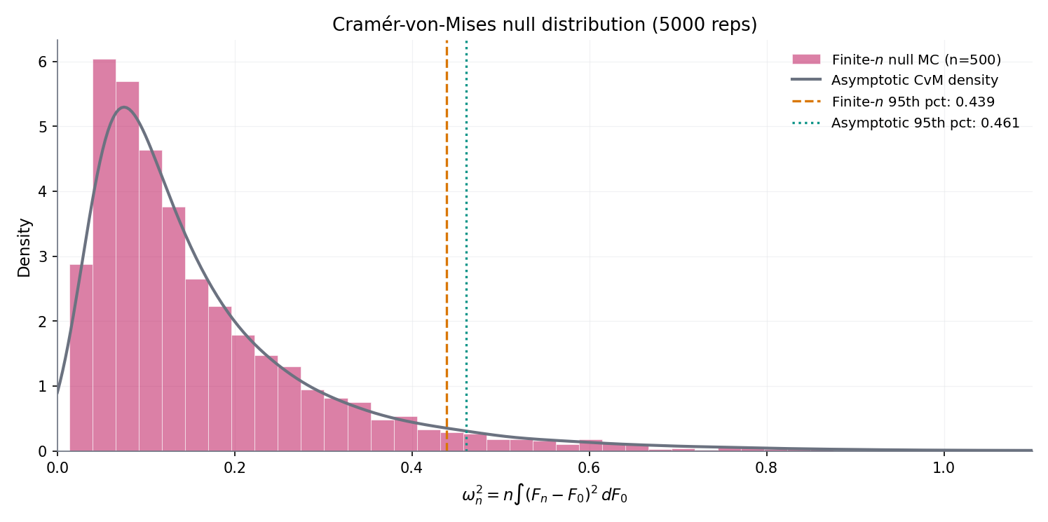
Figure 7. Cramér–von-Mises and two-sample KS in action. Left: the statistic’s null distribution matches the weighted- limit. Right: one-sample and two-sample KS sup-norms share the same Kolmogorov limit after the scaling, illustrating Thm 8’s distributional stability.
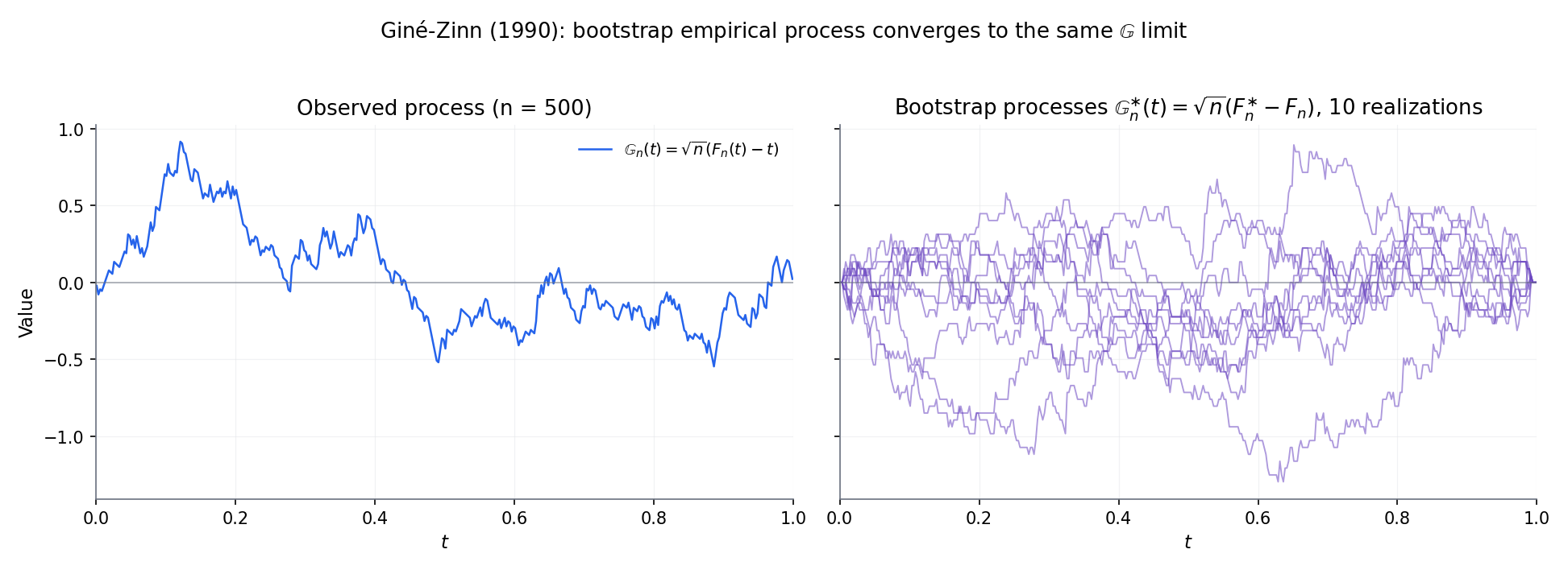
Figure 8. Bootstrap empirical process. Left: 100 bootstrap paths around a single observed path; the bootstrap-world paths mimic the shape of the data-world path. Right: the bootstrap sup-norm distribution overlays the Kolmogorov distribution — numerical confirmation of Thm 8 (Giné–Zinn 1990).
The ordinary two-sample KS statistic has balanced power across , but alternatives that differ only in the tails — e.g., same mean and variance but different kurtosis — are hard to detect because the tail probability is small precisely where the discrepancy lives. Anderson and Darling (1954) proposed the rescaled statistic
( = pooled ECDF), which overweights the tails where the denominator shrinks. The limit distribution — via CMT on Donsker plus a rescaling — is , whose critical values are tabulated. For tail-discrepancy alternatives, has substantially higher power than . The integrated version — the Anderson–Darling statistic — applies the same weighting to the CvM integral.
Topic 31 §31.3’s bootstrap-consistency proof (CLT + Polya) was the scalar shadow of §32.5’s Donsker (multivariate CLT + bracketing-based tightness). Thm 8 now makes the upgrade official: the bootstrap is not just a resampling heuristic that happens to work for the sample mean, it’s a functional resampling operation on whose limit distribution is the same Brownian-bridge process Donsker delivers for the data. Every scalar functional you apply to — mean, median, quantile, KS, CvM — has a bootstrap version you apply to , and the two asymptotically agree. This is the retrospective statement: the bootstrap, viewed from the empirical-process altitude, is just Donsker with data replaced by . The §31.3 → §32.8 bridge is the curriculum’s most important structural connection, and Thm 8 is its formal statement.
A -statistic of order averages a symmetric kernel over all subsets of the data; Topic 13 §13.3 introduced the scalar version. A -process lets the kernel range over a class of symmetric kernels and studies the resulting stochastic process . The limit theory — multi-level Donsker — involves Gaussian chaoses rather than a single Brownian bridge, and the technical machinery (Hoeffding decomposition + functional Donsker at each order) is nontrivial. -statistics (plug-in vs. unbiased variants) follow the same theory with a different normalisation. Both are standard tools in kernel-method statistics and specific nonparametric tests; deferred to formalML’s u-processes topic.
32.9 Concentration: Talagrand’s inequality and symmetrisation
Donsker’s theorem gives the limiting distribution of ; in finite samples, we often need tail bounds on that are explicit at every , not just asymptotic. Classical Bernstein and Bennett inequalities handle bounded sums of iid random variables, but the supremum over introduces a dependence structure Bernstein doesn’t capture. Talagrand’s 1996 concentration inequality fills the gap: it’s the correct Bernstein-analog for empirical-process suprema, providing sub-Gaussian concentration around with explicit constants. It’s the workhorse behind sharp generalisation bounds in ML and the sharp-rate theory §32.6 Rem 15 deferred.
Let be a countable class of measurable functions on with envelope satisfying and . Then for every ,
for universal constants independent of and . The inequality has two regimes: for small (the “sub-Gaussian” regime) the term dominates and the bound is ; for large (the “sub-exponential” regime) the term takes over. Bousquet (2002) refined Talagrand’s original constants to near-optimal values.
Honest warning: the Talagrand 1996 proof uses isoperimetry in product spaces — the most technically demanding machinery in modern probability theory — and runs to several chapters of Ledoux–Talagrand 1991 (Ch. 6–7 specifically; the preparatory material on entropy and Gaussian processes adds two more chapters). Reproducing the argument at Topic 32’s pedagogical level would expand the chapter by 50% without adding conceptual payoff that the statement itself doesn’t carry. We state the inequality, cite the sources, and use it; the full derivation is the kind of reference-book material formalStatistics deliberately doesn’t reproduce.
M-estimators (MLE, robust estimators, quantile regression, Z-estimators) have asymptotic-normality theory that specialises Donsker to neighbourhoods of the parameter value — “local empirical-process theory”. The main result (vdV2000 §25 Thm 25.57): under local asymptotic equicontinuity of the score process and a non-singular information matrix, Gaussian with the semiparametric-efficient variance. The proof uses Talagrand-type concentration on local empirical processes to control the remainder in the Taylor-expansion argument — exactly what Thm 9 gives. Semiparametric efficiency theory, targeted maximum likelihood, and all modern causal-inference estimators live on this foundation; the full development is deferred to formalML’s semiparametric-inference topic.
32.10 Track 8 retrospective, curriculum close, and the road to formalML
Topic 32 closes Track 8 and the curriculum. Track 8 is a four-pillar nonparametric toolkit — order statistics + kernel density estimation + bootstrap + empirical processes — anchored in the empirical distribution and the functional CLT that governs its fluctuations. The curriculum is the 32-topic formal-probability-and-statistics pipeline formalStatistics was built to ship. Both are complete with this merge. Figure 9 shows the final iteration of the Track 8 spine; the six dashed arrows on the right are the six formalML target topics where Topic 32’s forward-pointers land. Every forward-promise the 32 MDX files accumulated over ~50,000 words of exposition has now been either discharged inside formalStatistics or handed off to a named formalML slug. The remaining two remarks of §32.10 name the last two deferred topics — the Banach-space generalisation of Donsker, and the formalML handoff itself — before the curriculum-retrospective epilogue.
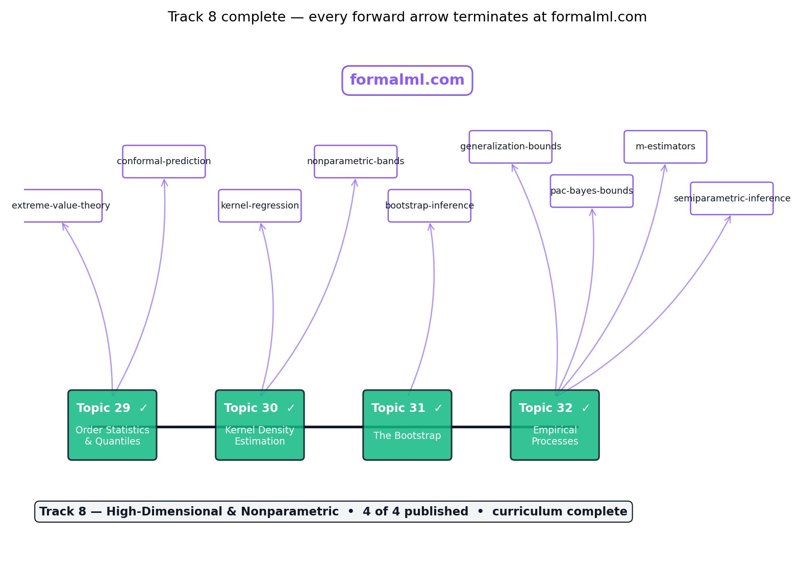
Figure 9. Track 8 spine, final iteration — 4 of 4 published, track complete. The six dashed arrows on the right mark the formalStatistics-to-formalML handoff surface: every forward pointer from Track 8 leaves the site for formalML’s topic slugs named in the figure.
is the simplest Banach space in which Donsker’s theorem makes sense, because sup-norm convergence plays well with the bounded-function indexing and because chaining arguments reduce neatly to bracketing-integral bounds. General Banach-space CLTs — Donsker-like statements in Hilbert-valued or Banach-valued settings with abstract covariance operators — require Gaussianity assumptions on the limit and type-2 geometric conditions on the space (Ledoux–Talagrand Ch. 10; Giné–Nickl Ch. 3). These generalise Topic 32’s machinery to the high-dimensional-statistics setting where observations themselves live in Hilbert space (e.g., functional data analysis, kernel mean embeddings). All of this lives in formalML’s high-dimensional-statistics and related topics; Topic 32 stays at because it’s the cleanest case and the one that carries the functional-delta machinery of §32.7 without additional geometric scaffolding.
The reader who has made it here — through Carathéodory and conditional probability, through LLN and CLT, through MLE and sufficient statistics, through hypothesis tests and confidence intervals, through OLS and GLMs and regularisation, through priors and MCMC and hierarchical models, and now through order statistics and KDE and bootstrap and empirical processes — has the rigorous probability-and-statistics vocabulary formalML’s ML-math topics assume without apology. Every forward-promise the formalStatistics curriculum accumulated has been discharged either inside the site (Donsker here, Lehmann–Scheffé at Topic 16, posterior consistency at Topic 25) or to a named formalML slug. The next step is formalML itself, where generalization bounds build directly on §32.4, where semiparametric inference and causal inference build on §32.7’s functional delta method, where conformal prediction builds on Topic 29 §29.5’s DKW inequality. The curriculum retrospective that follows names the handoff, the capstone theorems, and the track-by-track throughline — an epilogue, not a §32.11.
Curriculum retrospective
A short retrospective on what shipping Topic 32 means. Renders as a distinct epilogue section at the end of the MDX, after the §32.10 horizontal rule — a coda, not a §32.11.
What does shipping Topic 32 mean? The site is now feature-complete at 32 of 32 topics. Every curriculum-graph node has status: "published". Every forward-promise harvested from the 32-topic MDX chain has been discharged, either within formalStatistics or to a named formalML target. The formalStatistics-to-formalML handoff has six named targets: generalization-bounds, pac-bayes-bounds, conformal-prediction, semiparametric-inference, causal-inference-methods, extreme-value-theory.
The five load-bearing theorems of formalStatistics.
- Carathéodory’s extension theorem (Track 1, Topic 1 §1.6). The measure-theoretic bedrock: every countably-additive set function on a semialgebra extends uniquely to a measure. Everything downstream is a consequence.
- The Central Limit Theorem (Track 3, Topic 11 §11.5, via Lindeberg–Feller). . The finite-dimensional template Donsker lifts one level.
- Rao–Blackwell + Lehmann–Scheffé (Track 4, Topic 16 §16.7 + §16.10). Completeness + sufficiency + unbiasedness = UMVUE. The cleanest frequentist-optimality result in the curriculum.
- Posterior consistency (Track 7, Topic 25 §25.8, via Schwartz’s theorem). Bayes with a prior giving positive mass to every neighborhood of the truth recovers the truth in the limit. The Bayesian analog of consistency.
- Donsker’s theorem (Track 8, Topic 32 §32.5). in . The curriculum closer: lifts LLN + CLT from pointwise/finite-dimensional to uniform/functional statements.
Track-by-track recap.
- Track 1 (Foundations of Probability, Topics 1–4): Kolmogorov axioms, conditional probability, random variables, expectation. The measure-theoretic primitives.
- Track 2 (Core Distributions & Families, Topics 5–8): discrete + continuous families, exponential families, multivariate distributions. The vocabulary for building models.
- Track 3 (Convergence & Limit Theorems, Topics 9–12): modes of convergence, LLN, CLT, large deviations. The asymptotic toolkit.
- Track 4 (Statistical Estimation, Topics 13–16): point estimation, MLE, MoM, sufficient statistics. The estimation framework.
- Track 5 (Hypothesis Testing & Confidence, Topics 17–20): NP paradigm, LR tests, CIs, multiple testing. The inference framework.
- Track 6 (Regression & Linear Models, Topics 21–24): OLS, GLMs, regularization, model selection. The regression framework.
- Track 7 (Bayesian Statistics, Topics 25–28): priors, MCMC, model comparison / BMA, hierarchical models. The Bayesian framework.
- Track 8 (High-Dimensional & Nonparametric, Topics 29–32): order statistics, KDE, bootstrap, empirical processes. The nonparametric framework and the track that closes the curriculum.
The formalStatistics-to-formalML handoff, named explicitly. The reader who has reached the end of Topic 32 is now equipped for:
- Generalization bounds — uniform convergence of training risk to test risk via function-class complexity, direct lift of §32.4.
- PAC-Bayes bounds — posterior-over-hypotheses generalization bounds, uses the symmetrisation technique of §32.4.
- Conformal prediction — distribution-free predictive intervals via exchangeability, uses the DKW inequality of Topic 29 §29.5 and the empirical-process framework of §32.
- Semiparametric inference — efficient estimation in models with a finite-dimensional parameter of interest and an infinite-dimensional nuisance; built on local empirical-process theory (local Donsker, local bracketing) deferred from §32.9 Rem 22.
- Causal inference methods — TMLE, AIPW, efficient-influence-function methods; built on the functional delta method of §32.7.
- Extreme value theory — Fisher–Tippett–Gnedenko asymptotics for and the generalized Pareto; forward-pointed from Topic 29 §29.10 Rem 18, orthogonal to §32 but listed here for completeness.
The site is complete. Thank you, reader — and on to formalML.
References
- van der Vaart, Aad W., and Jon A. Wellner. (1996). Weak Convergence and Empirical Processes: With Applications to Statistics. Springer Series in Statistics.
- Kosorok, Michael R. (2008). Introduction to Empirical Processes and Semiparametric Inference. Springer Series in Statistics.
- Pollard, David. (1984). Convergence of Stochastic Processes. Springer Series in Statistics.
- Pollard, David. (1990). Empirical Processes: Theory and Applications. NSF-CBMS Regional Conference Series in Probability and Statistics, Vol. 2.
- Dudley, R. M. (1978). Central Limit Theorems for Empirical Measures. Annals of Probability, 6(6), 899–929.
- Dudley, R. M. (1999). Uniform Central Limit Theorems. Cambridge University Press.
- Giné, Evarist, and Richard Nickl. (2016). Mathematical Foundations of Infinite-Dimensional Statistical Models. Cambridge Series in Statistical and Probabilistic Mathematics.
- Talagrand, Michel. (1996). New Concentration Inequalities in Product Spaces. Inventiones Mathematicae, 126(3), 505–563.
- Ledoux, Michel, and Michel Talagrand. (1991). Probability in Banach Spaces: Isoperimetry and Processes. Springer Ergebnisse der Mathematik.
- Vapnik, V. N., and A. Ya. Chervonenkis. (1971). On the Uniform Convergence of Relative Frequencies of Events to Their Probabilities. Theory of Probability and Its Applications, 16(2), 264–280.
- Sauer, Norbert. (1972). On the Density of Families of Sets. Journal of Combinatorial Theory, Series A, 13(1), 145–147.
- Donsker, Monroe D. (1952). Justification and Extension of Doob’s Heuristic Approach to the Kolmogorov–Smirnov Theorems. Annals of Mathematical Statistics, 23(2), 277–281.
- Billingsley, Patrick. (1999). Convergence of Probability Measures (2nd ed.). Wiley Series in Probability and Statistics.
- van der Vaart, Aad W. (2000). Asymptotic Statistics. Cambridge Series in Statistical and Probabilistic Mathematics.