Empirical Bayes
Learning the prior from the ensemble. Topic 28 fit a Normal prior's two hyperparameters; Topic 33 leaves the prior unrestricted and either bypasses it — Robbins' formula and Tweedie's formula — or estimates it outright with the Kiefer–Wolfowitz NPMLE. Six full proofs: Tweedie's formula (featured), the compound-decision theorem, Robbins' formula, exponential-family Tweedie, the selection invariance of the Bayes rule, and the average coverage of empirical-Bayes intervals. Auto-insurance claims and 6,033 prostate-cancer z-scores as the spine datasets; the winner's curse, local false discovery rates, and the score-matching identity behind diffusion models as the ML payoff. The nonparametric coda to Track 7.
33.1 Motivation: the winner’s curse
Suppose we tune a model by trying 1,000 hyperparameter configurations and scoring each one once on a held-out validation set. The configuration at the top of the leaderboard looks excellent. Score it again on fresh data and it almost always looks worse. Nothing is wrong with that configuration; what went wrong is the ranking. Every validation score is a true quality plus noise, and the top of a ranked list is exactly where the noise has piled up in the flattering direction. This is the winner’s curse, and it is the oldest problem empirical Bayes solves.
Here is the notation we’ll use for the rest of the topic. Write for the true score of configuration — what we would see with an infinitely large validation set — and for the score we actually observed. The simplest honest model of the noise is
independently across . Read as “the error is drawn from a Normal distribution with mean 0 and variance .” We treat the noise level as known; for a validation accuracy computed on examples it is about . Equivalently, : given the true score, the observation scatters symmetrically around it. Throughout, is an expectation (a probability-weighted average) and is a variance (the average squared distance from the mean). The true scores themselves vary across configurations according to some distribution — most configurations are mediocre, a few are good — and is exactly what we will not know.
Take configurations whose true scores follow — 90% baseline configurations clustered near 0 and 10% genuinely better ones near 2.5 — with validation noise . Rank by observed score and keep the top 20. On average, their observed scores overstate their true scores by +1.41.
Two corrections, previewed here and justified in §33.4–§33.5:
- The oracle Bayes rule , which knows , overstates the top 20 by only +0.08.
- Tweedie’s formula with an estimated marginal — a Gaussian kernel density estimate (bandwidth ) fit to the 1,000 observed scores, with unknown — overstates them by +0.21.
The leaderboard also hides an impostor: the configuration at rank 13 has true score 0.47. It is a baseline configuration that got lucky on the validation draw.
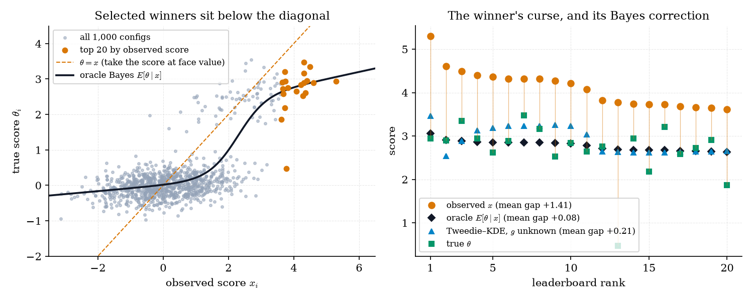
Figure 1. The winner’s curse on a simulated leaderboard. Selected winners sit below the diagonal; the oracle Bayes rule and Tweedie’s formula with an estimated marginal both deflate them.
The second spine dataset is genomic. Singh et al. (SIN2002) measured the expression of 6,033 genes on 102 men — 50 healthy controls and 52 prostate-cancer patients. For each gene, a two-sample -statistic converted to a -score measures how differently that gene behaves in the two groups (the file ships with EFR2016). A gene with no effect has ; a gene with effect has, to a good approximation, . The largest of the 6,033 -scores is . How big is that gene’s effect, really? It was selected because it is the largest, so, like the leaderboard winner, it is almost certainly overestimated. We answer the question in §33.5 Example 8.
When we face many parallel estimation problems at once — thousands of genes, hundreds of model configurations, every policy holder in an insurance book — the ensemble of observations carries information about the prior that no single observation does, and empirical Bayes is the discipline of learning that prior from the data it governs. Topic 28 did the parametric half, fitting a Normal prior’s two hyperparameters by Type-II maximum likelihood; Topic 33 takes the nonparametric half, where the prior is left unrestricted and is either bypassed (f-modeling: Robbins’ formula and Tweedie’s formula) or estimated outright (g-modeling: the Kiefer–Wolfowitz NPMLE). The organizing picture is geometric: under Normal noise the Bayes rule is the identity plus a shrinkage vector field equal to the score of the marginal density, , so every correction points uphill on and can be estimated without ever naming . That one identity explains why the best-looking model on a leaderboard is overestimated and how to deflate it, why James–Stein is a special case rather than a paradox, why local false-discovery rates are an empirical-Bayes computation, and why a diffusion model’s denoiser is trained by score matching.
The spine of the topic runs Robbins (§33.3) → Tweedie (§33.4–§33.5) → the nonparametric MLE of the prior (§33.6), then compares the two strategies (§33.7), re-reads large-scale testing as empirical Bayes (§33.8), and ends with what empirical-Bayes confidence intervals do and do not promise (§33.9).
Topic 28 learned the two hyperparameters of a Normal prior by maximizing the marginal likelihood — Type-II maximum likelihood, §28.7. James–Stein (§28.5) was the striking special case: shrinking Normal means toward a common point beats the MLE for every configuration of the means. Nothing here re-proves any of that. What changes is that is no longer forced to be Normal — it can be spiky, skewed, or multimodal, which is what real ensembles of effects look like. One notational change: Topic 28’s groups become this topic’s parallel problems, because will grow large and asymptotics in are the point.
Robbins (ROB1956) coined the phrase. A single problem’s Bayes rule needs a prior , and with one observation there is no way to check it. But a large ensemble of parallel problems, each drawing its parameter from the same , carries its own information about : the histogram of the is a blurred picture of . The prior stops being a statement of belief and becomes an estimable population distribution — the distribution of true effects across genes, of true quality across configurations, of true accident rates across drivers.
33.2 The compound decision problem
Before estimating anything we need to say what “good” means when we estimate parameters at once. The frame is Robbins’ compound decision problem (ROB1951): many parameters, one estimation rule applied to all of them, judged by average error. That is the situation of a hyperparameter sweep, an experimentation platform running thousands of A/B tests, or a recommender estimating a click-through rate for every item in the catalog.
Fix real numbers — no prior, just unknown constants — and observe independent , . A separable rule applies one function to every coordinate: . Its compound risk is the average mean squared error
where averages over with held fixed.
For a prior on the parameter, the Bayes rule is the posterior mean , computed with and . With — the empirical distribution that puts mass on each true parameter — is the oracle Bayes rule (EFR2019’s “oracle Bayes”): it would be available only to someone who knew the histogram of the . An empirical-Bayes rule is any rule built from the data to estimate , and its regret is .
This is where most readers lose the thread, so let’s slow down. Nothing in Definition 1 is random except the noise. The are fixed, and the compound risk is a purely frequentist quantity: an average over hypothetical re-draws of the noise. Yet the theorem below says the best separable rule is a posterior mean — a Bayesian object — under a particular prior, . The prior was never assumed; it falls out of the averaging over . Part (ii) of the proof treats that average as an iterated integral, first over given the parameter and then over the parameter drawn from , which is the order-of-integration bookkeeping of formalCalculus: Multiple Integrals & Fubini's Theorem .
Let be fixed real numbers and let be independent with . For a separable rule with finite compound risk, and with the empirical distribution of the parameters:
(i) the compound risk equals the Bayes risk of under the prior ,
(ii) for every separable , where
with equality if and only if almost everywhere under the marginal .
Proof 1 Proof of Thm 1 (fundamental theorem of compound decisions) [show]
(i) For any function , the average is the integral of against , because puts mass on each . Apply this to .
(ii) Introduce a random pair with and . By (i), the compound risk is the joint expectation
Condition on and write . For fixed , expanding and taking the conditional expectation — the cross term has conditional mean zero — gives
Averaging over with the tower property,
The second term does not depend on ; the first is nonnegative and vanishes exactly when almost everywhere under the law of , which is . Finally, Bayes’ theorem with the discrete prior (mass at each ; the cancels) gives . — using the tower property of conditional expectation and Bayes’ theorem for a discrete prior (ROB1951; ZHA2003).
Theorem 1 turns estimation into a target. The best we can do with a separable rule is ; we can’t compute it, because it depends on the unknown , but every empirical-Bayes method is an attempt to estimate it from the . The two families of attempts differ in what they estimate.
f-modeling estimates the marginal density of the observations (or a functional of it, such as its log-derivative) and plugs the estimate into a formula for the Bayes rule that depends on only through . g-modeling estimates the prior itself and computes the Bayes rule of the estimate.
Restrict attention to linear rules with Normal noise, . For each coordinate, is a mean-zero noise term plus a constant, so its mean square is . Averaging over ,
For fixed , the second term is the average squared distance between and the points , minimized at their mean: , where . Substituting, with the spread of the true parameters,
Setting the derivative in to zero, , gives . The best linear rule is therefore , with shrinkage fraction .
Now estimate the two unknowns. Replace by , and estimate by . Under Normal-prior sampling, , the observations are marginally , so ; since , the estimator has expectation exactly . The result is the Efron–Morris rule (EFR1973),
James–Stein is not a paradox: it is the empirical-Bayes estimate of the best linear separable rule. Nonparametric empirical Bayes drops the word “linear.”
No prior was assumed anywhere in Theorem 1 — the are fixed — and yet the optimal separable rule is a posterior mean under . Robbins called procedures that approach this optimum without knowing “asymptotically subminimax” (ROB1951): for large they do nearly as well as if the histogram of the true parameters had been revealed. Separable rules are the natural class because the problems are exchangeable before we see the data — nothing distinguishes problem 7 from problem 700. A non-separable rule can beat only by exploiting the ordering of the indices, which carries no information when the labels are arbitrary.
Figure 2 shows why the two strategies are genuinely different. A prior can be spiky — here, three point masses — but the data never see it directly. They see the marginal : the prior convolved with (smeared by) the Normal noise, which is always smooth. f-modeling works with that smooth object; g-modeling tries to undo the smearing. f-modeling is Robbins’ formula (§33.3) and Tweedie’s formula (§33.4–§33.5); g-modeling is the nonparametric MLE of the prior (§33.6); §33.7 compares them head to head.
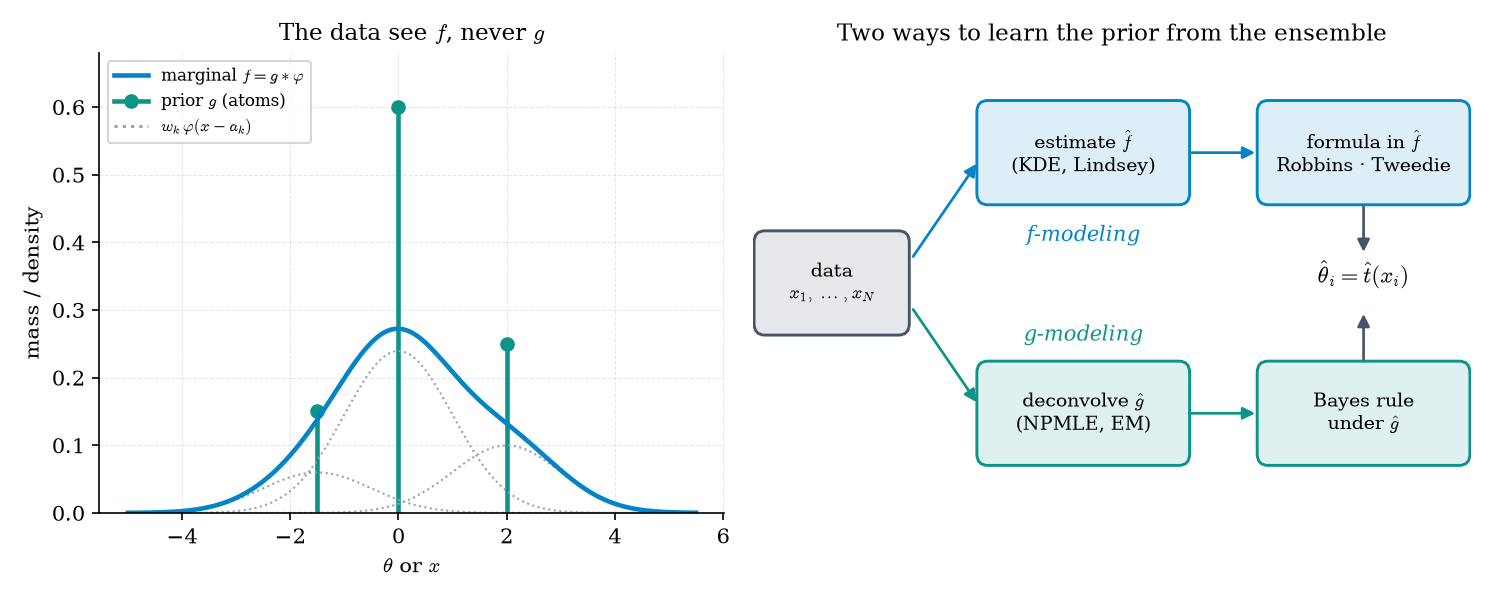
Figure 2. The data see the marginal f, never the prior g. f-modeling estimates f and plugs it into a formula; g-modeling deconvolves an estimate of g and computes its Bayes rule.
33.3 Robbins’ formula
Robbins’ first example was insurance. Each policy holder has an unknown accident rate — expected claims per year — and the number of claims in a year is , the standard model for counts of rare, independent events. Rates vary across the book according to an unknown distribution on . The marginal probability is the fraction of all holders with exactly claims, and it is directly visible in the data. The same structure governs per-user event counts in a product — clicks, purchases, sessions — and the question Robbins answered is the cold-start question: what should we predict next period for a user we observed times this period?
Let , any probability measure on , and , with marginal
Then for every with ,
Proof 2 Proof of Thm 2 (Robbins' formula) [show]
By Bayes’ theorem the posterior is , so
Multiply and divide the integrand by , using :
Dividing by gives the formula. — using Bayes’ theorem and the Poisson pmf (ROB1956).
The prior has disappeared. Replacing by the empirical frequency , where is the number of holders with exactly claims, gives Robbins’ estimator , in which cancels. For each fixed with , the frequencies and converge almost surely to and by the strong law of large numbers (Topic 10), and the ratio converges because it is a continuous function of them away from .
CASI Table 6.1 (EFR2016) records one year of claims for 9,461 policy holders of a European auto insurer:
| Claims | 0 | 1 | 2 | 3 | 4 | 5 | 6 | 7 |
|---|---|---|---|---|---|---|---|---|
| Holders | 7840 | 1317 | 239 | 42 | 14 | 4 | 4 | 1 |
| Robbins | 0.168 | 0.363 | 0.527 | 1.33 | 1.43 | 6.00 | 1.75 | — |
These are identical to CASI’s published row. The first entry is the cold-start answer: customers with no claims this year should expect claims next year — not 0, which is what the MLE says. Customers with one claim should expect 0.363, far less than 1: one claim is weak evidence of a high rate, because most of the book has low rates and some of them file a claim by chance.
The parametric alternative assumes a shape for : with shape and scale . Then the posterior given is , with mean
and the marginal of is negative binomial. Its maximum-likelihood fit preserves the sample mean, , so the fit reduces to a one-dimensional profile in , which gives and . The fitted rule for is
0.164, 0.398, 0.632, 0.866, 1.100, 1.334, 1.568
(CASI: .164 .398 .633 .87 1.10 1.34 1.57). Figure 3 puts the two side by side: they agree where the counts are large, and Robbins goes erratic where they are small.
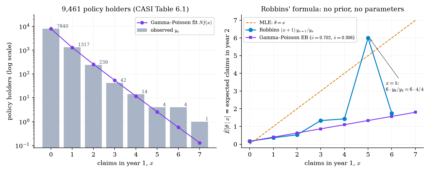
Figure 3. Robbins’ formula on 9,461 insurance policy holders. It needs no prior and no parameters, and it is erratic exactly where the counts are small.
The explorer below puts both rules next to each other on the insurance data and on a simulated book where the true posterior mean is known. Click a count bar to perturb that count by ±1 and watch which estimates move.
| x | yₓ | Robbins | Gamma EB |
|---|---|---|---|
| 0 | 7840 | 0.168 | 0.164 |
| 1 | 1317 | 0.363 | 0.398 |
| 2 | 239 | 0.527 | 0.632 |
| 3 | 42 | 1.333 | 0.866 |
| 4 | 14 | 1.429 | 1.100 |
| 5 | 4 | 6.000 | 1.334 |
| 6 | 4 | 1.750 | 1.568 |
At , Robbins’ estimate is : two tiny counts drive it. A single extra policy holder with six claims would change it to . The parametric fit borrows strength across every ; Robbins borrows only from the neighboring cell . The explorer’s perturbation buttons make the difference tactile — perturbing moves Robbins at and substantially and leaves the Gamma rule essentially unchanged.
For the Poisson family, is nondecreasing in for every prior. The posterior at is the posterior at tilted by a factor of , so
because . This is the discrete twin of §33.4 Theorem 3(iii). Robbins’ drop from 6.00 at to 1.75 at is therefore an estimation artifact, not a feature of any prior. We’ll turn this observation into a diagnostic in §33.7.
33.4 Tweedie’s formula (featured)
Now return to the setting of §33.1: Normal noise with known variance and an arbitrary prior . Write
for the density — the bell curve of the noise — and for the standard Normal density. The marginal density of an observation is , written : the prior smeared out by the noise. Let . Its derivative is the score of the marginal — the slope of the log-density, which tells us which way, and how steeply, the data pile up. Robbins (ROB1956) credits the next result to Maurice Tweedie; Efron’s “Tweedie’s formula and selection bias” (EFR2011) is the modern treatment. It is the Normal-noise version of Robbins’ formula, and it is the featured result of this topic.
Let be any probability measure on , , and with known. Write and
Then is strictly positive and twice differentiable, and for every :
(i) ;
(ii) ;
(iii) — the Bayes rule is nondecreasing in .
Proof 3 Proof of Thm 3 (Tweedie's formula) [show]
Step 0 — differentiating under the integral. The -derivatives of the integrand are
Both are bounded functions of , because is bounded for . A bounded function is integrable against the probability measure , so dominated convergence lets us differentiate twice under the integral sign ( formalCalculus: The Lebesgue Integral , Ex 10). The integrand is strictly positive, so and is well defined.
Step 1 — the mean. By Step 0,
The posterior is , so dividing by turns the integral into a posterior expectation:
Multiplying by and adding gives (i).
Step 2 — the variance. Again by Step 0 and the same division,
Since and ,
where the last step uses that shifting by the constant does not change its conditional variance. Multiplying by and rearranging gives (ii).
Step 3 — monotonicity. Differentiating (i) gives , which equals by (ii), and a variance is nonnegative. — using dominated convergence (formalCalculus: The Lebesgue Integral) and Bayes’ theorem (ROB1956; EFR2011).
Read (i) geometrically. The Bayes rule is the identity map plus a correction, and the correction is a vector field on the line: at each point it says which way the marginal density increases and how fast. Figure 4 draws it.
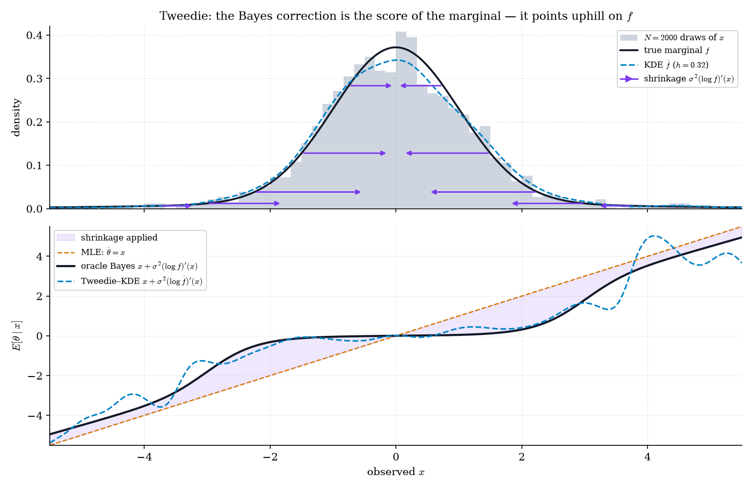
Figure 4. Tweedie’s formula as geometry: the Bayes correction is σ² times the score of the marginal, a field of arrows pointing uphill on f. Bottom: the resulting nonlinear shrinkage rule, oracle versus KDE estimate.
The explorer makes the field live. Choose a prior, change the sample size and the bandwidth, and compare the KDE-estimated rule to the oracle. Try the Normal prior first: the oracle rule becomes a straight line, which is Topic 28’s linear shrinkage (Example 5 below). Then shrink or the bandwidth and watch the estimated rule wiggle in the tails.
| MLE (x) | 0.997 |
| Tweedie–KDE | 0.207 |
| Oracle Bayes | 0.168 |
Tweedie–KDE recovers 95% of the oracle's improvement over the MLE.
Take . The marginal is — a Normal prior smeared by Normal noise is Normal with the variances added — so
Tweedie’s formula returns with , and part (ii) gives the posterior variance . This is exactly Topic 28’s partial-pooling formula (§28.6, Thm 4), now a one-line special case. The rule is linear because is quadratic; every non-Normal prior bends it.
Take — 90% of the effects are exactly zero, the rest are spread widely — with and draws. The oracle rule at is 0.047, 0.316, 1.805, 4.498: near-total shrinkage near 0, where an observation is most likely a null plus noise, and near-identity in the tails, where it is most likely a real effect.
For the f-modeling estimate, fit a Gaussian KDE (Topic 30) with Silverman’s bandwidth : . Differentiating term by term and dividing by , the KDE score has the closed form
a softmax-weighted pull toward nearby data points. Per-coordinate mean squared error on the sample: the MLE scores 1.033, Tweedie–KDE 0.244, the oracle 0.193. With unknown, Tweedie–KDE captures about 94% of the oracle’s improvement over the MLE.
Part (i) says the correction points toward higher marginal density. Observations in sparse regions get pulled toward where the data are dense — Figure 4’s arrows all point at the spike. The noise variance sets the step size: noisier measurements are pulled harder, because they say less about their own . That is the whole content of shrinkage, stated without a prior.
The rule depends on only through , which is what makes f-modeling possible: estimate from the , differentiate its logarithm, done. The price is that we need a derivative of a density estimate, and derivative estimates are noisy where data are thin — Example 6’s KDE rule wiggles in the tails. Bandwidth controls the trade-off exactly as in Topic 30: see the MISE/AMISE analysis in §30.5 and data-driven bandwidth selection in §30.8.
Corrupt a clean sample with Gaussian noise, with . Theorem 3 in — the proof runs coordinate by coordinate — gives
where is the density of the noisy samples. A denoiser trained by squared error, minimizing , converges to the posterior mean , so estimates the score . That is denoising score matching (VIN2011), the training objective behind score-based diffusion models: every denoising network is an f-modeling estimate of Tweedie’s correction. formalML’s representation-learning topic develops the identity (§3.4 there, Thm 3.2): formalML: representation-learning .
33.5 Tweedie beyond the Normal, and selection bias
Tweedie’s formula is not special to Normal noise. Any one-parameter exponential family (Topic 7) has the same structure: the posterior mean of the natural parameter is a log-derivative of the marginal, corrected by the carrier. This matters in ML because many of the quantities we shrink are not Normal — counts, rates, variances.
Let be a one-parameter exponential family of densities on an open interval , in Topic 7’s notation (natural parameter , cumulant function , carrier twice differentiable on ). Let , a probability measure on the natural parameter space with for every . With and :
(i) ; (ii) .
Proof 4 Proof of Thm 4 (exponential-family Tweedie) [show]
Factor the carrier out of the marginal:
so and it suffices to show and . For in a compact sub-interval , gives , so () is dominated by a -integrable function not depending on . Dominated convergence ( formalCalculus: The Lebesgue Integral ) then justifies
The posterior is — the carrier cancels. Hence and , so
Substituting gives (i) and (ii). — using dominated convergence, as in Thm 3, and the exponential-family representation of Topic 7 (EFR2011).
Check that Theorem 4 contains Theorem 3. The Normal density factors as , so the natural parameter is , the cumulant function is , and the carrier is , with and . Part (i) reads , which is Theorem 3(i) after multiplying by ; part (ii) reads , which is Theorem 3(ii).
For an integer-valued family , derivatives in are replaced by shifts. Dividing the marginal by the carrier,
and the ratio of the two is a posterior expectation, because the posterior given is proportional to :
For the Poisson family, , so , , and , which makes . The display becomes — Theorem 2.
To use Tweedie’s formula on real data we need an estimate of . The KDE of Example 6 is one choice. A second, which Efron uses for the prostate data, fits a smooth exponential family to the histogram.
Bin the data into equal-width bins with centers , width , and counts . Fit the Poisson regression
where is the standardized bin center, and set . The estimated score is the derivative of a polynomial — smooth everywhere. The fit is exactly the Poisson generalized linear model of Topic 22, with histogram counts as the response.
Now the selection question. The top genes were chosen because their -scores were large, and the winning configuration was chosen because its validation score was largest. Does choosing on the data invalidate the posterior mean? It does not.
Let , , be independent pairs with and , and let . Let be any selection rule that is a function of — the indices of the largest , or all with . Then for every with ,
Proof 5 Proof of Thm 5 (selection invariance of the Bayes rule) [show]
Independence of the pairs means is conditionally independent of given , so the other coordinates carry no information about once is known:
The indicator is a function of , so it can be pulled inside a conditional expectation given . By the tower property,
Dividing by gives the conditional statement. — using the tower property and conditional independence (DAW1994; EFR2011).
By contrast, when selects large — that is the winner’s curse of §33.1. Selection biases the naive estimate, not the posterior mean. The posterior mean already accounts for the fact that a large is more likely to be a moderate plus favorable noise than a large , and that accounting doesn’t care why we are looking at this particular .
Fit Lindsey’s method to the 6,033 prostate -scores with 90 bins on and degree . The leading coefficient is negative, so the fitted density is integrable, and across the data range, so the estimated rule is monotone, as Theorem 3(iii) says a Bayes rule must be. For the ten largest -scores:
| 5.29 | 4.83 | 4.47 | 4.40 | 4.25 | 4.19 | 4.14 | 4.12 | 4.10 | 3.98 | |
|---|---|---|---|---|---|---|---|---|---|---|
| 4.64 | 3.86 | 3.26 | 3.14 | 2.90 | 2.80 | 2.72 | 2.71 | 2.67 | 2.49 |
The top gene’s effect is estimated at 4.64, not 5.29; the tenth gene’s at 2.49, not 3.98. Is this really Efron’s? A cross-check: with the theoretical null and null proportion 1, the local false discovery rate flags 51 genes (26 right, 25 left) — EFR2008’s count exactly.
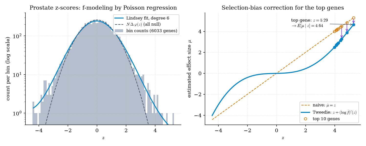
Figure 5. Lindsey’s method on the prostate z-scores, and Tweedie’s selection-bias correction for the top genes: the largest z-score, 5.29, deflates to an estimated effect of 4.64.
Return to Example 1, now with unknown, as it always is in practice. Fit a Gaussian KDE to the 1,000 observed scores themselves and apply Tweedie’s formula: the top-20 overstatement falls from +1.41 to +0.21 (the oracle, which knows , gets +0.08). The practical recipe for a sweep:
- Standardize each configuration’s validation score by its sampling standard deviation — for an accuracy, — so that the noise is approximately .
- Fit a KDE (or Lindsey’s method) to the standardized scores and apply .
- Report the corrected score of the leader, not its raw score; by Theorem 5, the correction stays valid even though we selected the leader on the data.
The explorer below runs the experiment. The default scenario is Example 1’s; averaged over the default draw and the next 19 resamples, the implementation here gives naive +1.27, Tweedie–KDE +0.13, and oracle −0.04 — the oracle sits near zero, as Theorem 5 predicts — and a single resample varies around those values. Raise the validation noise and watch the curse get worse and the correction get larger.
| Naive (x) | +1.02 |
| Tweedie–KDE | +0.02 |
| Oracle Bayes | −0.23 |
Theorem 4 covers the Gamma and chi-square families as well, which is how one shrinks thousands of sample variances at once — the idea behind moderated -statistics in genomics (the limma approach), where each gene’s variance estimate borrows strength from all the others. Poisson rates are covered through Example 7. The structure is always the same: estimate the marginal, take a log-derivative, correct by the carrier.
The KDE continues Topic 30 and needs no model, but its score oscillates in sparse tails, where only a few data points contribute to the softmax weights. Lindsey’s polynomial is smooth and extrapolates sensibly, but it needs a degree choice: to is standard, and EFR2011 uses natural splines with 5 degrees of freedom and a sixth-degree polynomial in its examples. The interactive components in this topic use KDE; the prostate figures use Lindsey.
Theorem 5 needs the true . Empirical Bayes estimates , so the immunity is inherited only approximately; EFR2011 gives the empirical evidence that it holds up well in practice. The frequentist alternative keeps fixed and builds intervals that are valid conditional on the selection event — selective inference: formalML: selective-inference . The two answer different questions: selective inference controls error over repetitions of the selection, while the posterior mean averages over the ensemble of effects that produced the data.
33.6 g-modeling: the nonparametric MLE of the prior
f-modeling sidesteps the prior. g-modeling goes straight at it: find the prior that makes the observed data most likely, over all priors. This is maximum likelihood (Topic 14) over an infinite-dimensional parameter — a probability measure.
The nonparametric maximum-likelihood estimator of the prior is
where the maximum is over all probability measures on . The objective is concave in : is linear in , and the logarithm of a linear function is concave.
Let have distinct values, and with over all probability measures on . (a) attains its maximum, and the fitted values are the same for every maximizer . (b) Some maximizer is discrete with at most support points, all in . (c) maximizes if and only if the gradient function
satisfies for all , with equality at every support point of .
The intuition for (c): is the directional derivative of the concave average log-likelihood in the direction of a point mass at . At the optimum, no direction improves it, so everywhere; and moving mass off a support point can’t help either, which forces there (LIN1983).
(a) (Kiefer–Wolfowitz 1956.) If i.i.d. and , then weakly, almost surely. (b) (Jiang–Zhang 2009.) Under mild moment conditions on the unknown means, the rule (“general maximum likelihood empirical Bayes”) has compound risk — asymptotically as good as the oracle separable rule of Theorem 1 — provided that oracle risk is of larger order than .
Part (b) is the payoff of the whole compound-decision frame: the NPMLE rule achieves the benchmark of Theorem 1 without knowing , for essentially any configuration of the means. Part (a) says the estimated prior converges too, but weakly — in the sense of distribution functions, not densities — which is why we judge g-modeling by its rule rather than by how looks.
Computing the NPMLE. Restrict to a fixed grid on with weights summing to 1. The EM algorithm (LAI1978) updates
The factor multiplying is exactly the gradient function of Theorem 6: EM raises the weight of every grid point where and lowers it where , and its fixed points have wherever . Each step increases the likelihood, and we stop when — the certificate of Theorem 6(c). The empirical-Bayes rule is then
a genuine Bayes rule for the prior , and therefore monotone by Theorem 3(iii).
Take — three types of unit, with no spread within a type — with , , a 181-point grid on , and 20,000 EM steps. The estimated mass concentrates in three clusters near the true atoms, with cluster masses 0.07 / 0.66 / 0.26 (true 0.15 / 0.60 / 0.25), and : the Theorem 6(c) certificate is satisfied. The fit is not perfect, and it shouldn’t be — the atoms at and are only apart, so at the data can’t fully separate them, and some of the atom’s mass is absorbed by the atom at 0.
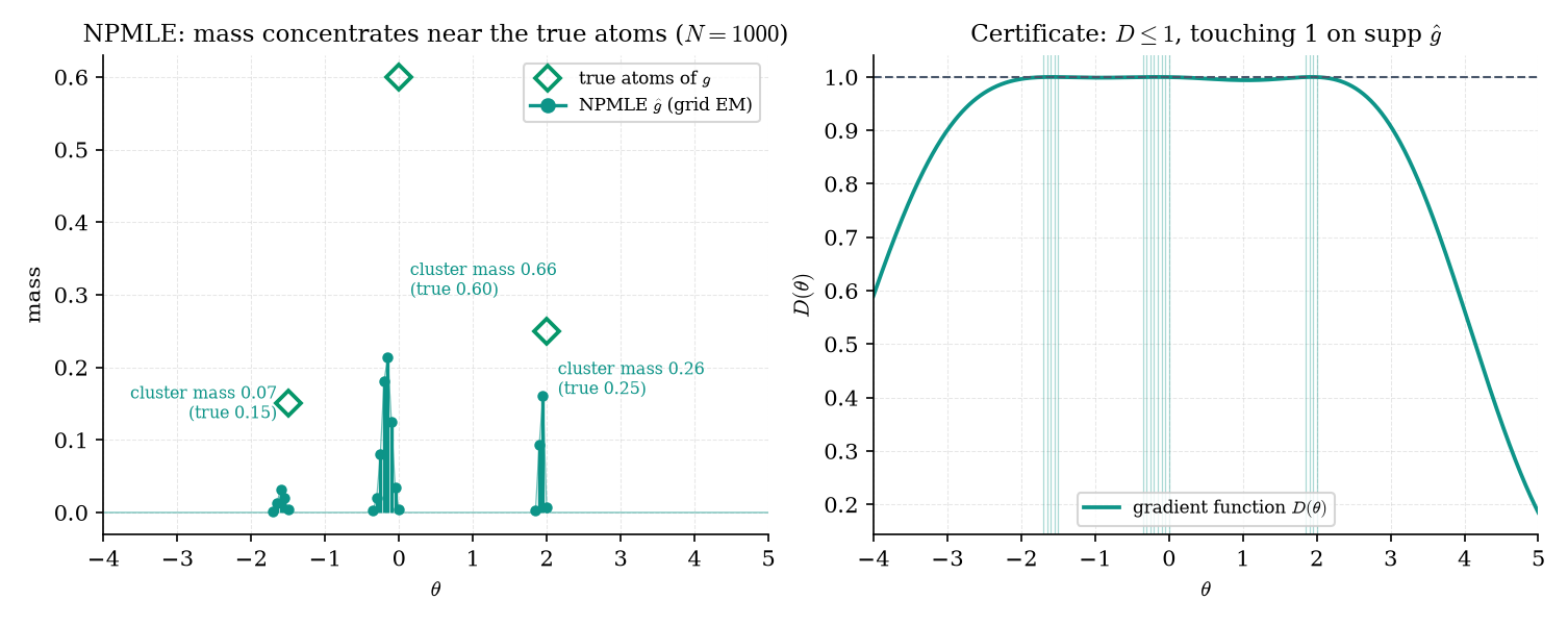
Figure 6. g-modeling: the NPMLE concentrates its mass near the true atoms, and the gradient function certifies optimality by touching 1 exactly on its support.
The fitter below runs the EM live. Step it a few times from the uniform start, then run it to the certificate and watch the gradient function settle onto the line . The bottom panel compares the resulting NPMLE rule with Tweedie–KDE and the oracle.
EM smears mass over adjacent grid points — Example 10’s fit has 17 support points, not 3 — and converges sublinearly, which is why it needed 20,000 steps. On a fixed grid the problem is a finite-dimensional convex program, and interior-point methods solve it exactly in seconds (KOE2014; the R package REBayes). We use EM here because each step is one line, it is monotone, and it can be paused and resumed — which is what the fitter’s step buttons need.
Theorem 6(b) makes discrete even when the true is continuous — try the Normal preset in the fitter. That is not a defect. The rule is still a smooth function of , because it averages the atoms with Gaussian weights, and Theorem 7(b) is a statement about the rule, not about .
Topic 28 Remark 11 pointed “a nonparametric empirical-Bayes prior” toward formalML. The NPMLE is that object, and it lives here: James–Stein shrinks toward an implicitly estimated Normal prior, while g-modeling estimates the prior with no shape restriction at all. Positive-part James–Stein and the Baranchik family themselves remain Topic 28’s (§28.5).
33.7 f-modeling versus g-modeling
We now have two complete empirical-Bayes strategies. Which is better? The question matters in practice because the two disagree exactly where the decisions are made: in the tails, where the interesting genes and the winning configurations live.
Take a sparse prior with — most effects are exactly zero, a few sit well above it — and run 40 replications for each . Regret is the per-coordinate mean squared error of each rule minus that of the oracle Bayes rule under the true , on the same sample:
| 100 | 200 | 500 | 1000 | 2000 | 5000 | |
|---|---|---|---|---|---|---|
| MLE | 0.7952 | 0.7802 | 0.7829 | 0.7897 | 0.7668 | 0.7681 |
| Positive-part James–Stein | 0.2525 | 0.2564 | 0.2558 | 0.2501 | 0.2474 | 0.2482 |
| Tweedie–KDE | 0.1416 | 0.0958 | 0.0656 | 0.0456 | 0.0286 | 0.0196 |
| NPMLE–EB | 0.0647 | 0.0336 | 0.0180 | 0.0096 | 0.0033 | 0.0025 |
The MLE’s regret does not shrink with : it never learns anything from the ensemble. Positive-part James–Stein’s regret is flat too, at about 0.25 — linear shrinkage cannot adapt to sparsity, because no single shrinkage factor is right both for the zeros and for the effects near 3. The two nonparametric rules learn the prior: Tweedie–KDE’s regret falls from 0.142 to 0.020, and the NPMLE rule’s from 0.065 to 0.0025.
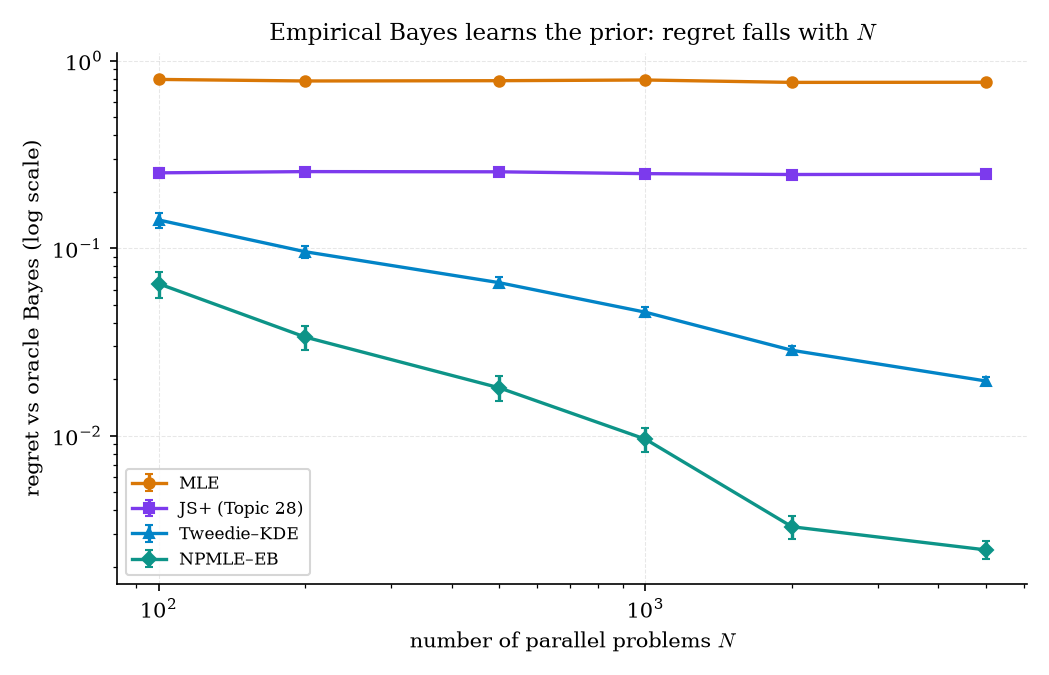
Figure 7. Regret against the oracle Bayes rule. Empirical Bayes learns the prior — Tweedie–KDE and NPMLE regret fall with N — while the MLE and linear shrinkage stay flat.
Theorem 3(iii) gives a cheap diagnostic that needs no oracle: every Bayes rule is nondecreasing. An estimated rule that decreases somewhere cannot be the Bayes rule for any prior, so wherever it decreases it is wrong.
Restrict to , which contains the 223 genes with , and compare three empirical-Bayes rules. The Tweedie–KDE rule (bandwidth ) is wildly non-monotone, with minimum slope : it maps to 1.20 while mapping to 2.35, so a larger observed effect gets a smaller estimated effect. Tweedie–Lindsey is monotone (minimum slope 0.57). The NPMLE rule is monotone (minimum slope 0.02) and saturates near 2.7, because the largest atom of sits at about 2.7 — a posterior mean can never exceed the largest value the prior allows. For the top gene, Lindsey estimates 4.64 and the NPMLE 2.72.
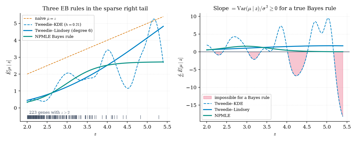
Figure 8. Every Bayes rule is monotone. In the sparse prostate tail the KDE-based rule is not; Lindsey’s smooth fit and the NPMLE rule are — but they disagree about how far to shrink.
In the bulk of the data all three rules agree. In the sparse tail, f-modeling extrapolates the shape of — Lindsey’s polynomial keeps bending at the rate it bent where data were plentiful — while g-modeling refuses to place prior mass where no cluster of data supports it, and so caps the estimate at its largest atom. Neither is “right” from 223 tail genes. EFR2019 discusses the oracle-Bayes benchmark and why g-modeling’s extra structure usually wins on regret (Example 11), while f-modeling is easier to compute and to explain. A good habit: when the two disagree about the decision you care about, report both.
Brown and Greenshtein (BRO2009) show that kernel f-modeling with a slowly shrinking bandwidth has vanishing relative regret, so the KDE route is asymptotically sound; Example 12’s pathology is a finite-sample problem. Koenker and Mizera (KOE2014) repair it directly: imposing monotonicity of the rule — equivalently, convexity of — turns the KDE estimate into a convex program whose solution is always a legitimate Bayes-rule shape.
33.8 Large-scale inference as empirical Bayes
Topic 27 introduced the two-groups model for thousands of simultaneous tests (§27.9). Each -score comes from the null with probability and from a non-null distribution otherwise, so the marginal density is , and the local false discovery rate
is the posterior probability that a case with score is null — a Bayes quantity. Topic 27 assumed the three ingredients were known: , the null density , and . Here we estimate all three from the 6,033 genes. That estimation step is empirical Bayes, and it is how screening at scale — genomics, fraud flags, A/B-test portfolios — is done in practice.
Fit a quadratic to the log of the estimated marginal on a central interval ( here), where nearly all cases are null, and match it to the log of a scaled Normal, , where is the density. Matching the coefficients of , , and gives
Central matching on the Lindsey fit of Example 8 gives (−0.001, 1.060, 0.980); EFR2008 reports . The null is centered where theory says, but it is 6% wider than . That small change matters a great deal. Counting genes with : the theoretical null flags 51 (26 right, 25 left); the empirical null flags 21 (13 right, 8 left). A 6% wider null removes more than half of the discoveries, because the discoveries live in the tails, where a slightly wider null puts a lot more null mass.
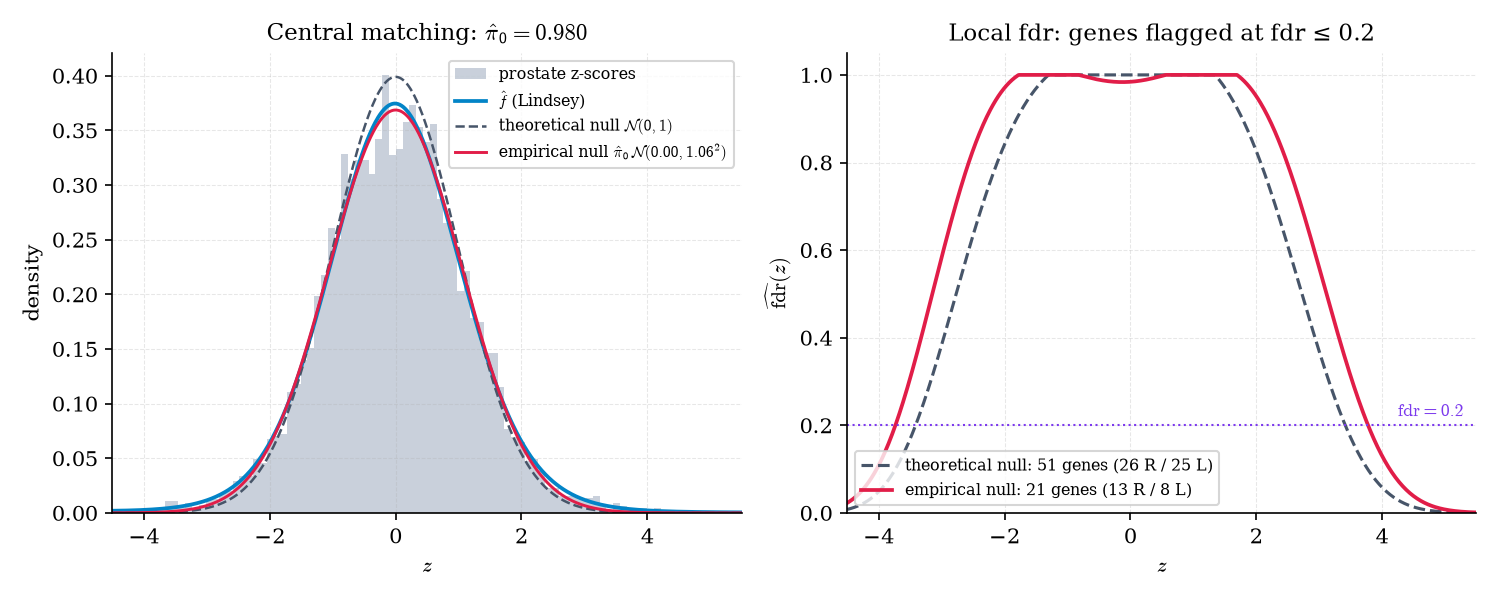
Figure 9. Large-scale inference as empirical Bayes: an empirical null fit by central matching is 6% wider than N(0,1) and cuts the genes at fdr ≤ 0.2 from 51 to 21.
The Benjamini–Hochberg procedure of Topic 20 looks like a purely frequentist device. It is also an empirical-Bayes estimate.
Define the tail-area false discovery rate , where and are the survival functions of under the mixture and under the null: the posterior probability that a case is null given that its score is at least as extreme as . Estimate each piece crudely: ; , the two-sided -value; and the empirical survival function at the -th smallest -value. Then
Benjamini–Hochberg rejects the hypotheses with the smallest -values, where
which is the largest tail region whose empirical-Bayes estimate of the Fdr is at most . On the prostate data with , BH rejects 60 genes. The frequentist guarantee — FDR control under independence — is Topic 20’s §20.7 Theorem 5 (Topic 20); the empirical-Bayes reading explains why the procedure has the form it has.
Topic 27 derived the local fdr with a theoretical null and a known mixture. The only new content here is estimating , , and from the ensemble — and that is exactly the empirical-Bayes step. Topic 27’s LocalFDRExplorer already exposes a theoreticalNull: false switch (Topic 27 Remark 24); central matching is the estimator behind it.
Correlation among genes, unobserved covariates that affect many genes at once, and miscalibrated test statistics all widen the central peak of the -score histogram, and Efron’s analyses find all three at work in microarray data. The empirical null absorbs them without our having to model them. Correlation-adjusted inference proper is out of scope for this topic.
33.9 Empirical-Bayes confidence intervals
Point estimates are half the job. Per-item uncertainty — an interval for each gene’s effect, each item’s click-through rate, each user’s treatment effect — is the other half, and it is where empirical Bayes is most often misused. Topic 28 Remark 16 said that empirical-Bayes intervals are “too narrow.” This section makes that precise, and shows the sense in which they are not. We need two more pieces of notation: is the standard Normal cumulative distribution function, and is its quantile ().
In the Normal–Normal model with known and shrinkage factor , the parametric empirical-Bayes confidence interval (EBCI) is
Its conditional coverage at is , a frequentist probability with held fixed. Its average coverage is — equivalently, the long-run fraction of the intervals that cover their own .
Let and with known, , , , , and . Then:
(i) , the probability taken over jointly;
(ii) for fixed with and ,
(iii) and as .
Proof 6 Proof of Thm 8 (average and conditional coverage of the parametric EBCI) [show]
(i) By Topic 28 §28.6 Thm 4, . Hence, for every value of , with ; averaging over leaves .
(ii) Fix . Rewrite the estimation error as a noise part and a bias part:
Given , , so . Standardizing by gives . The interval covers exactly when , that is, when
and for .
(iii) At , and , because . As , and both terms tend to the same limit (both to 1 if , both to 0 if ), so . — using the Normal–Normal posterior (Topic 28 §28.6 Thm 4).
A consistency check ties (ii) back to (i). Averaging over makes , since . Unconditionally, then, , and — part (i) again, by direct computation. The two parts together say what “too narrow” means: the interval is exactly right on average across units, and it pays for that by overcovering units near the prior mean and badly undercovering units far from it.
The parametric guarantee leans on the prior being Normal. Armstrong, Kolesár, and Plagborg-Møller (ARM2022) keep only its variance.
Let with , and define the normalized bias , the non-coverage function for , and
With the value of solving : (a) for every distribution of with — so that — the interval has average coverage at least ; (b) writing and ( when ),
attained by the distribution putting mass at and split equally at when . The parametric EBCI of Theorem 8 corresponds to the smaller critical value .
The intuition: once only the variance of is pinned down, nature can choose the prior that hurts the interval most, and the worst case piles most units exactly at the prior mean (where the interval overcovers, wasting nothing) and puts a few far out (where it undercovers badly). The robust critical value is the smallest one that survives that adversary (ARM2022, §2 and Prop. B.1).
Take , so and the parametric half-width is . Conditional coverage at (in units of ) is 0.994, 0.962, 0.780, 0.410, while the average is exactly 0.95. A unit three prior standard deviations from the mean — a genuine outlier, the kind we most want to get right — is covered 41% of the time.
The robust critical value is 3.259, so the robust half-width is , 18% wider than the parametric one. Average coverage under three priors, all with variance :
| Prior | Parametric | Robust |
|---|---|---|
| Normal | 0.950 | 0.979 |
| Spike-and-slab | 0.955 | 0.966 |
| Least favorable: mass 0.889 at , 0.111 split at | 0.929 | 0.950 |
The parametric interval’s average guarantee breaks under the least-favorable prior; the robust interval’s holds for all three.
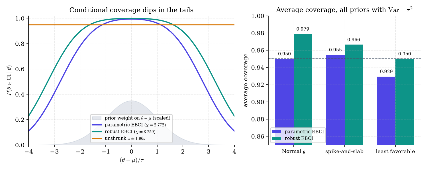
Figure 10. Empirical-Bayes intervals cover on average but not individually: conditional coverage dips in the tails, and robust intervals keep the average guarantee for every prior with the right variance.
Topic 28’s Type-II MLE on the eight-schools data (§28.7, Example 9) found . Then for every school, and every plug-in EBCI collapses to the single point with zero width — the extreme case of “too narrow.” Plug-in robust EBCIs inherit the problem, since . The fix is to account for the uncertainty in (Remark 20) or to go fully Bayes with a weakly informative hyperprior (Topic 28 Remark 17).
Theorem 8 assumed known. In practice they are estimated, and the plug-in interval ignores that error. Morris (MOR1983) inflates the interval with an analytic correction for estimating the hyperparameters; Laird and Louis (LAI1987) use a parametric bootstrap — the “corrected EB” workflow Topic 28 Remark 16 named. Nonparametric EBCIs that drop the Normal-prior assumption altogether (Ignatiadis and Wager) are beyond this topic.
Across all priors with the right variance and all shrinkage levels, the parametric EBCI’s average non-coverage can reach at (ARM2022, Lemma 4.1) — 74% coverage for a nominal 95% interval. Adding a constraint on the kurtosis of the prior narrows the robust interval (ARM2022, §3). The ML reading: per-item uncertainty for shrunken estimates — per-arm click-through rates in a bandit, per-user treatment effects, per-segment conversion rates — should be reported with robust EBCIs, not plug-in posterior intervals, whenever there is no strong reason to believe the effects are Normally distributed.
33.10 Forward look
The spine of this topic is one idea in five forms. Robbins showed that a large ensemble can stand in for an unknown prior, and that for Poisson counts the Bayes rule can be read off the marginal frequencies. Tweedie’s formula did the same for Normal noise and made the picture geometric: the Bayes correction is times the score of the marginal, a field of arrows pointing uphill on , which is why it deflates the winner’s curse and why it survives selection. The NPMLE estimated the prior outright and, through the compound-decision theorem, achieved the oracle’s risk without knowing the oracle’s prior. Large-scale testing turned out to be the same computation applied to the null, and empirical-Bayes intervals turned out to promise average coverage across units — no more, and no less. Topic 28 remains the closer of Track 7’s core arc; this topic is its nonparametric coda, and the remaining threads lead to formalML.
g-modeling maximizes over priors. The fully Bayesian alternative puts a prior on the prior — a Dirichlet process on — and integrates over it instead of maximizing. Dirichlet-process mixtures are the Bayesian counterpart of the NPMLE, with posterior uncertainty about built in: formalML: bayesian-nonparametrics .
In meta-learning, many related tasks play the role of the parallel problems, and the learned initialization or prior plays the role of : training across tasks estimates the prior, and adapting to a new task shrinks its estimate toward what the prior expects. formalML’s meta-learning topic develops the parametric (Type-II) version in its §6.3; this topic supplies the nonparametric toolkit and the compound-decision justification: formalML: meta-learning .
Everything here assumed a common noise level . Real ensembles rarely cooperate: Efron and Morris’s baseball batting averages (EFR1975) already had unequal sample sizes, and shrinkage with unequal is done well by minimizing Stein’s unbiased risk estimate (SURE; XIE2012). The NPMLE extends to multivariate parameters and to heteroskedastic noise, and nonparametric empirical-Bayes intervals are an active research area. Each is a natural next step from the tools of this topic.
References
- Robbins, Herbert. (1956). An Empirical Bayes Approach to Statistics. In Proceedings of the Third Berkeley Symposium on Mathematical Statistics and Probability, Vol. 1 (University of California Press), 157–163.
- Robbins, Herbert. (1951). Asymptotically Subminimax Solutions of Compound Statistical Decision Problems. In Proceedings of the Second Berkeley Symposium on Mathematical Statistics and Probability (University of California Press), 131–148.
- Zhang, Cun-Hui. (2003). Compound Decision Theory and Empirical Bayes Methods. Annals of Statistics, 31(2), 379–390.
- Efron, Bradley, and Carl Morris. (1973). Stein’s Estimation Rule and Its Competitors — An Empirical Bayes Approach. Journal of the American Statistical Association, 68(341), 117–130.
- James, Willard, and Charles Stein. (1961). Estimation with Quadratic Loss. In Proceedings of the Fourth Berkeley Symposium on Mathematical Statistics and Probability, Vol. 1 (University of California Press), 361–379.
- Efron, Bradley, and Trevor Hastie. (2016). Computer Age Statistical Inference: Algorithms, Evidence, and Data Science. Cambridge University Press.
- Efron, Bradley. (2011). Tweedie’s Formula and Selection Bias. Journal of the American Statistical Association, 106(496), 1602–1614.
- Vincent, Pascal. (2011). A Connection Between Score Matching and Denoising Autoencoders. Neural Computation, 23(7), 1661–1674.
- Dawid, A. Philip. (1994). Selection Paradoxes of Bayesian Inference. In Multivariate Analysis and Its Applications, IMS Lecture Notes–Monograph Series 24, 211–220.
- Efron, Bradley, and Robert Tibshirani. (1996). Using Specially Designed Exponential Families for Density Estimation. Annals of Statistics, 24(6), 2431–2461.
- Singh, Dinesh, Phillip G. Febbo, Kenneth Ross, et al. (2002). Gene Expression Correlates of Clinical Prostate Cancer Behavior. Cancer Cell, 1(2), 203–209.
- Kiefer, J., and J. Wolfowitz. (1956). Consistency of the Maximum Likelihood Estimator in the Presence of Infinitely Many Incidental Parameters. Annals of Mathematical Statistics, 27(4), 887–906.
- Laird, Nan. (1978). Nonparametric Maximum Likelihood Estimation of a Mixing Distribution. Journal of the American Statistical Association, 73(364), 805–811.
- Lindsay, Bruce G. (1983). The Geometry of Mixture Likelihoods: A General Theory. Annals of Statistics, 11(1), 86–94.
- Jiang, Wenhua, and Cun-Hui Zhang. (2009). General Maximum Likelihood Empirical Bayes Estimation of Normal Means. Annals of Statistics, 37(4), 1647–1684.
- Koenker, Roger, and Ivan Mizera. (2014). Convex Optimization, Shape Constraints, Compound Decisions, and Empirical Bayes Rules. Journal of the American Statistical Association, 109(506), 674–685.
- Brown, Lawrence D., and Eitan Greenshtein. (2009). Nonparametric Empirical Bayes and Compound Decision Approaches to Estimation of a High-Dimensional Vector of Normal Means. Annals of Statistics, 37(4), 1685–1704.
- Efron, Bradley. (2014). Two Modeling Strategies for Empirical Bayes Estimation. Statistical Science, 29(2), 285–301.
- Efron, Bradley. (2019). Bayes, Oracle Bayes and Empirical Bayes. Statistical Science, 34(2), 177–201.
- Efron, Bradley. (2004). Large-Scale Simultaneous Hypothesis Testing: The Choice of a Null Hypothesis. Journal of the American Statistical Association, 99(465), 96–104.
- Efron, Bradley. (2008). Microarrays, Empirical Bayes and the Two-Groups Model. Statistical Science, 23(1), 1–22.
- Efron, Bradley. (2010). Large-Scale Inference: Empirical Bayes Methods for Estimation, Testing, and Prediction. Cambridge University Press.
- Morris, Carl N. (1983). Parametric Empirical Bayes Inference: Theory and Applications. Journal of the American Statistical Association, 78(381), 47–55.
- Laird, Nan M., and Thomas A. Louis. (1987). Empirical Bayes Confidence Intervals Based on Bootstrap Samples. Journal of the American Statistical Association, 82(399), 739–750.
- Armstrong, Timothy B., Michal Kolesár, and Mikkel Plagborg-Møller. (2022). Robust Empirical Bayes Confidence Intervals. Econometrica, 90(6), 2567–2602.
- Efron, Bradley, and Carl Morris. (1975). Data Analysis Using Stein’s Estimator and Its Generalizations. Journal of the American Statistical Association, 70(350), 311–319.
- Xie, Xianchao, S. C. Kou, and Lawrence D. Brown. (2012). SURE Estimates for a Heteroscedastic Hierarchical Model. Journal of the American Statistical Association, 107(500), 1465–1479.