Sample Spaces, Events & Axioms
The Kolmogorov axioms — non-negativity, normalization, and countable additivity — define the contract that every valid probability distribution must satisfy
1. Experiments, Outcomes & Sample Spaces
Probability is the mathematics of uncertainty. Before we can assign probabilities to anything, we need a precise language for describing what could happen. That language starts with three terms:
- An experiment (or random experiment) is any process whose outcome is not known in advance.
- An outcome is one specific result of the experiment.
- The sample space is the set of all possible outcomes.
These are not deep concepts — they’re agreements about notation. But getting them right is essential, because every probability statement we’ll ever make is a statement about subsets of .
The sample space of a random experiment is the set whose elements are the possible outcomes of the experiment. An individual outcome is called a sample point.
Examples of Sample Spaces
Sample spaces range from the trivially finite to the uncountably infinite:
| Experiment | Sample Space | Size |
|---|---|---|
| Flip a fair coin | Finite, | |
| Roll a six-sided die | Finite, | |
| Roll two dice (ordered) | Finite, | |
| Flip a coin until heads | Countably infinite | |
| Pick a real number in | Uncountable | |
| Lifetime of a component | Uncountable |
The distinction between finite, countably infinite, and uncountable matters enormously — it determines which mathematical tools we need. For finite and countable spaces, we can sum. For uncountable spaces, we must integrate.
![Gallery of four sample spaces: coin flip, die roll, flip-until-heads, uniform [0,1]](/images/topics/sample-spaces/sample-spaces-gallery.png)
Use the explorer below to build sample spaces for different experiments and see how events and probabilities emerge:
2. Events as Sets
An event is any collection of outcomes — a subset of . We say event occurs if the actual outcome of the experiment satisfies .
An event is a subset . The event occurs if the outcome of the experiment belongs to .
Special events:
- The certain event always occurs.
- The impossible event never occurs.
- A simple event consists of a single outcome.
Let .
- is the event “roll an even number.”
- is the event “roll at least 5.”
- is the event “roll an even number that is at least 5.”
- is the event “roll an even number or at least 5.”
- is the event “do not roll an even number” (i.e., roll odd).
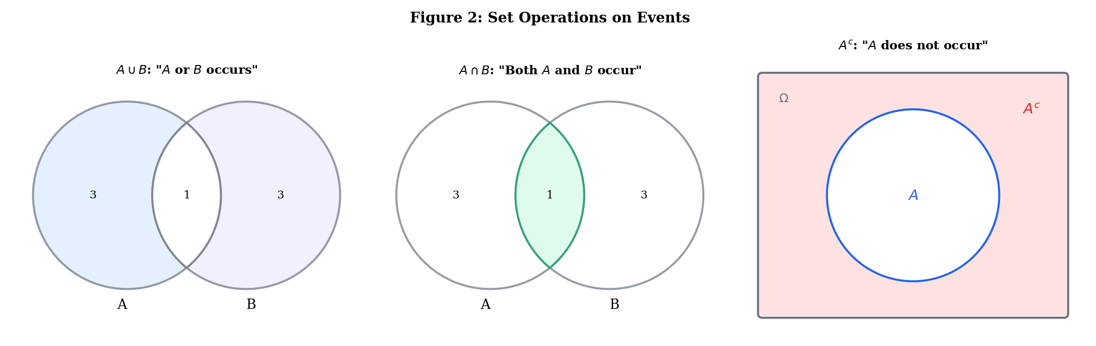
Set Operations as Logical Connectives
The correspondence between set operations and logical statements about events is exact:
| Set Operation | Notation | Meaning |
|---|---|---|
| Union | or (or both) occurs | |
| Intersection | Both and occur | |
| Complement | does not occur | |
| Set difference | occurs but does not | |
| Subset | If occurs, then occurs | |
| Disjoint | and cannot both occur |
De Morgan’s laws connect them:
In words: “not both” equals “not one or not the other,” and “neither” equals “not either.” De Morgan’s laws generalize to arbitrary collections of events — including countably infinite unions and intersections, which is where sigma-algebras enter the picture.
Explore set operations interactively — toggle different operations to highlight regions and see De Morgan’s laws in action:
3. Sigma-Algebras
The Problem with “All Subsets”
For finite sample spaces, life is simple: the collection of events is just the power set . With a six-sided die, has subsets, and we can assign a probability to each one without trouble.
For uncountable sample spaces like , things break. There is no way to assign a probability to every subset of while satisfying the Kolmogorov axioms — this is the content of the Vitali construction (1905), which produces a non-measurable set. The details require measure theory we’ll encounter in the Measure-Theoretic Probability topic on formalML: measure-theoretic probability .
The fix is elegant: instead of trying to assign probabilities to all subsets, we work only with a well-behaved collection called a sigma-algebra.
A -algebra (or -field) on a set is a collection satisfying:
- (the sample space is an event)
- If , then (closed under complements)
- If , then (closed under countable unions)
By De Morgan’s law, closure under complements + countable unions gives closure under countable intersections for free. And since , the empty set is always in .
The word “countable” in axiom (3) is doing heavy lifting. A collection closed under finite unions but not countable unions is called an algebra (or field) of sets. The upgrade from algebra to -algebra is exactly what we need for limit theorems — taking limits of sequences of events requires countable set operations.
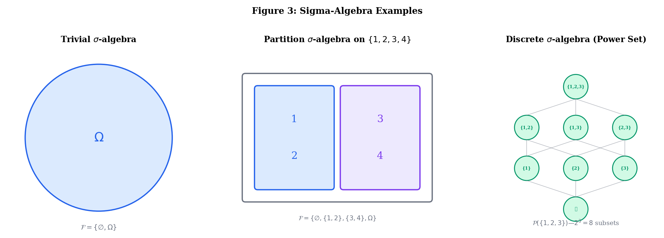
- The trivial -algebra is the smallest possible — we can only say “something happened” or “nothing happened.”
- The discrete -algebra is the largest — every subset is an event. This works for countable .
Let . Consider .
Check: (1) ✓. (2) ✓. (3) All unions of members yield members ✓.
This -algebra “sees” the partition but cannot distinguish 1 from 2 or 3 from 4. It encodes partial information — a theme that becomes central in conditional probability and filtrations.
On , the Borel -algebra is the smallest -algebra containing all open intervals . It contains all open sets, all closed sets, all countable intersections of open sets ( sets), all countable unions of closed sets ( sets), and more. This is the standard -algebra for probability on — the one you use 99% of the time.
Why this matters for ML: When you write ”,” you are implicitly working with the Borel -algebra on . The measurability requirement — that a random variable must pull Borel sets back to events in your -algebra — is what makes statements like "" well-defined. We’ll formalize this in Random Variables & Distribution Functions.
Build your own sigma-algebras below. Select subsets and watch the validator check the closure properties in real time:
4. The Kolmogorov Axioms
We now have the stage (), the actors (), and we need the script: a function that assigns a number to each event. Kolmogorov’s axioms (1933) tell us what properties this function must have.
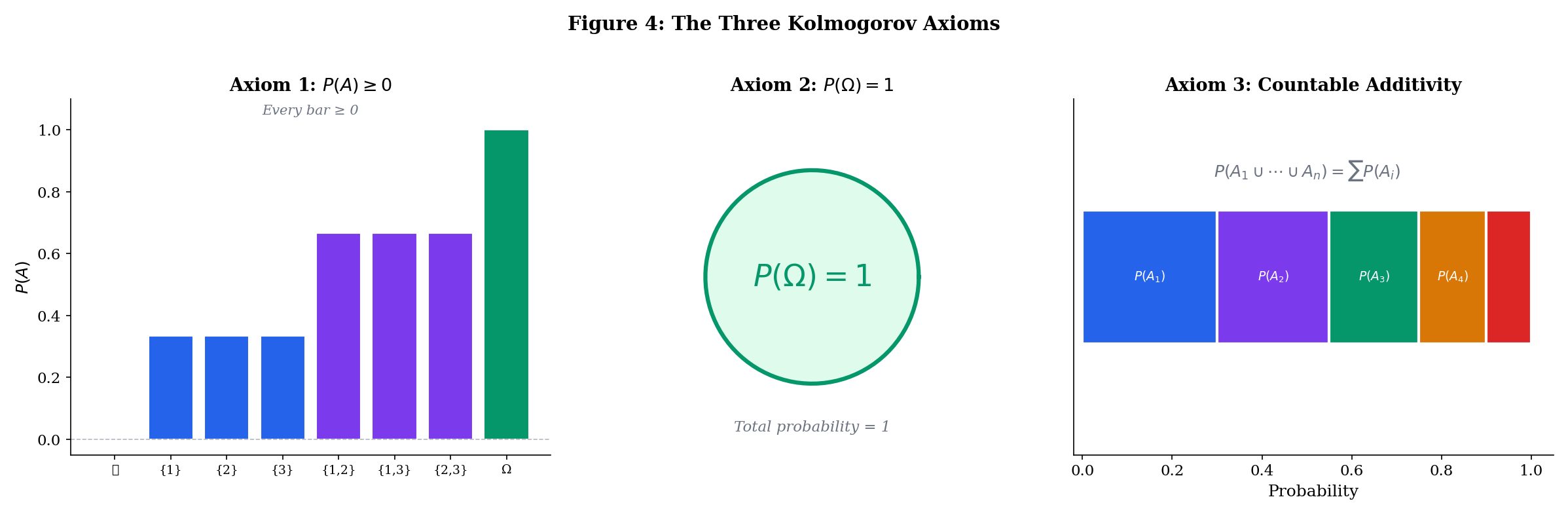
A probability measure on a measurable space is a function satisfying:
Axiom 1 (Non-negativity). For every , .
Axiom 2 (Normalization). .
Axiom 3 (Countable Additivity). If are pairwise disjoint (i.e., for all ), then
The triple is called a probability space.
That’s it. Three axioms. Every theorem in probability theory — the law of large numbers, the central limit theorem, Bayes’ rule, the convergence of your neural network’s training loss — follows from these three axioms plus the machinery of analysis.
Axiom 3 demands countable additivity, not mere finite additivity. This is the axiom that makes limit theorems possible. If we only required for finite collections, we could not take limits of sequences of events — and without limits, no convergence theorems, no law of large numbers, no central limit theorem. The jump from “finitely many” to “countably many” is small in notation but enormous in mathematical power.
Roll a fair die. The probability space is:
- (all 64 subsets)
- for each , extended by additivity:
Check the axioms: (1) ✓. (2) ✓. (3) For disjoint : ✓.
5. Consequences of the Axioms
Everything in this section is derived from the three axioms — no additional assumptions needed. This is the engine of probability theory: a small axiomatic base generating a rich body of results.
The Complement Rule
For any event ,
Proof [show]
Since and are disjoint and , Axiom 3 gives (by Axiom 2). Rearranging: .
.
Proof [show]
Take in Theorem 1: .
Monotonicity
If , then .
Proof [show]
Write , where and are disjoint. By Axiom 3:
since by Axiom 1.
The Addition Rule (Inclusion-Exclusion for Two Events)
For any events ,
Proof [show]
Decompose into three pairwise disjoint pieces:
By Axiom 3:
Now, (disjoint), so , giving . Similarly . Substituting:
General Inclusion-Exclusion
For events ,
The proof proceeds by induction on , with the base case being Theorem 3. The inductive step applies Theorem 3 to and uses the distributive law.
Step through the inclusion-exclusion formula term by term and watch the running total converge to the exact probability:
Adjust probabilities
Union Bound (Boole’s Inequality)
For any countable collection of events ,
Proof [show]
Define and for . The are pairwise disjoint, , and . By countable additivity and monotonicity:
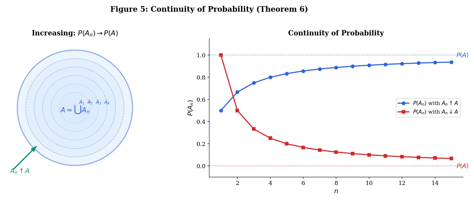
Continuity of Probability
Let .
(a) If (i.e., and ), then .
(b) If (i.e., and ), then .
Proof [show]
Proof of (a). Define and for . The are pairwise disjoint and . So . By countable additivity:
Proof of (b). Apply part (a) to , then use the complement rule.
This is where the convergence of sequences from formalCalculus: sequences & limits becomes essential — the telescoping sum and limit exchange are the same tools you developed there.
Given finite additivity, countable additivity is equivalent to continuity from below (Theorem 6a). This means Axiom 3 is really saying “probability is a continuous set function,” connecting our probability axioms directly to the continuity of limits.
6. Combinatorial Probability
The Equally Likely Model
When is finite and every outcome is equally probable — for all — probability reduces to counting:
This is the classical or Laplacian definition of probability. It’s a special case of the Kolmogorov axioms, not the foundation — many important probability spaces (continuous distributions, unfair coins) don’t have equally likely outcomes.
Counting Tools
To use the equally likely model, we need to count. The three essential counting principles:
Multiplication Principle. If experiment 1 has outcomes and experiment 2 has outcomes, the combined experiment has outcomes.
Permutations. The number of ways to arrange items chosen from (order matters) is .
Combinations. The number of ways to choose items from (order doesn’t matter) is .
The Birthday Problem
In a group of people, what is the probability that at least two share a birthday? Assume 365 equally likely birthdays.
It’s easier to compute the complement: .
- Person 1 has choices.
- Person 2 must avoid person 1’s birthday: .
- Person must avoid the previous birthdays: .
The famous result: with just people, the probability exceeds 50%.
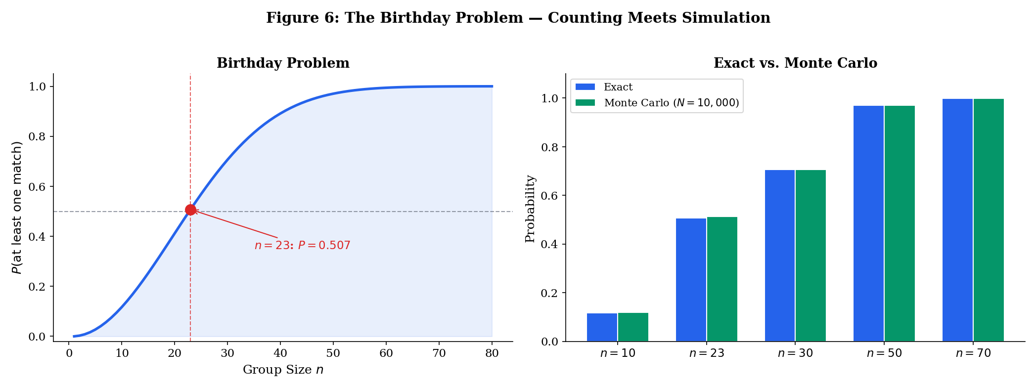
Explore the birthday problem below — adjust the group size and run Monte Carlo simulations to see the exact curve confirmed empirically:
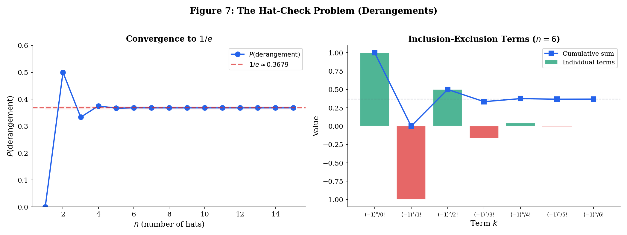
The Matching Problem (Derangements)
people check their hats; the hats are returned at random. What is the probability that nobody gets their own hat back?
A permutation with no fixed points is called a derangement. Let be the event “person gets their own hat.” We want .
By inclusion-exclusion:
So the probability of a derangement is:
This is remarkable: for large , the probability converges to , independent of . The convergence is extremely fast — already at , the answer is accurate to three decimal places.
7. Conditional Probability & Independence (Preview)
We close the mathematical content with a brief preview of the next topic. Conditional probability answers: “given that event has occurred, what is the probability of event ?”
For events with ,
Events and are independent if
Equivalently (when ): — knowing occurred doesn’t change the probability of .
These concepts are the subject of Conditional Probability & Independence. We’ll prove Bayes’ theorem, develop the law of total probability, and explore the surprisingly subtle concept of conditional independence — the assumption behind naive Bayes classifiers, graphical models, and essentially all tractable probabilistic inference.
8. Connections to ML
Probability Spaces in Disguise
Every ML model implicitly defines a probability space:
| ML Model | Sample Space | -Algebra | Probability |
|---|---|---|---|
| Bernoulli classifier | |||
| Multinomial (softmax) | Softmax output | ||
| Gaussian model | |||
| Language model | Token sequences | Cylinder -algebra | Autoregressive factorization |
| Diffusion model | Learned via score matching |
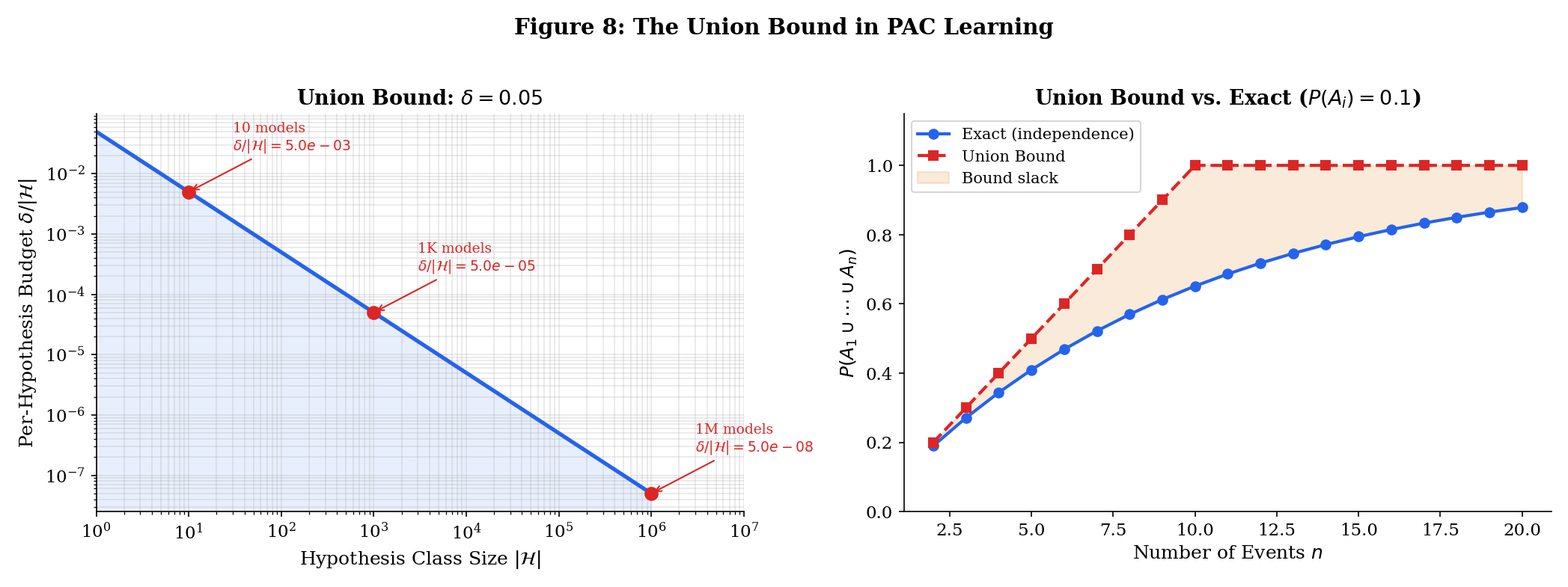
The Union Bound in Learning Theory
Boole’s inequality (Theorem 5) is the entry point to PAC learning. The core argument:
- You have hypotheses (models).
- For each , define = “hypothesis overfits” (training error is small but true error is large).
- You want .
- By the union bound: .
- So it suffices to make for each .
This is the simplest version of the uniform convergence argument. It tells you that generalization requires either few hypotheses or very tight per-hypothesis bounds — the fundamental tension of statistical learning theory. The full treatment lives on formalML: measure-theoretic probability .
Sigma-Algebras and Information
In Bayesian ML, the -algebra encodes what you can observe. A filtration models information arriving over time:
- In online learning, is the information available after seeing data points.
- In reinforcement learning, is the history up to time (all states, actions, rewards).
- In time series, is the natural filtration of the observed process.
This seems abstract now, but when we get to martingales and stochastic processes later in formalStatistics, filtrations will be the language we use to formalize “what the model knows at each step.”
9. Summary
| Concept | Key Idea |
|---|---|
| Sample space | The set of all possible outcomes |
| Event | A subset of outcomes; “something we can ask about” |
| -algebra | The collection of “askable” events — closed under complements and countable unions |
| Probability measure | A function satisfying non-negativity, normalization, and countable additivity |
| Probability space | The complete specification of a probabilistic model |
| Complement rule | |
| Addition rule | |
| Union bound | — the workhorse of PAC learning |
| Continuity | — why countable additivity matters |
| Combinatorial probability | when outcomes are equally likely |
What’s Next
The next topic — Conditional Probability & Independence — builds on this foundation to answer: “how does new information change probabilities?” We’ll derive Bayes’ theorem, formalize independence, and see why conditional independence is the structural assumption that makes probabilistic ML tractable.
References
- Billingsley, P. (2012). Probability and Measure (Anniversary ed.). Wiley.
- Durrett, R. (2019). Probability: Theory and Examples (5th ed.). Cambridge University Press.
- Grimmett, G. & Stirzaker, D. (2020). Probability and Random Processes (4th ed.). Oxford University Press.
- Wasserman, L. (2004). All of Statistics. Springer.
- Shalev-Shwartz, S. & Ben-David, S. (2014). Understanding Machine Learning: From Theory to Algorithms. Cambridge University Press.